REVIEW 3 major objections 5 minor 47 references
Scale-Consistent Learning for Partial Differential Equations
T0 review · 3 major / 5 minor · reviewed 2026-08-15 · deepseek-v4-flash
Pith's one-line read A neural PDE solver trained at one scale can generalize to unseen scales if it is trained to respect scale consistency, with a theorem showing that exact scale consistency plus accuracy on near-constant inputs pins down the true solution…
desk verdict A genuinely useful scale-consistency regularizer for neural operators, with a theory that is real but narrower than the abstract and a self-referential super-domain loss that needs to be honestly caveated. read the letter →
The pith
A machine-rendered reading of the paper's core claim, the machinery that carries it, and where it could break.
The reading
What carries the argument
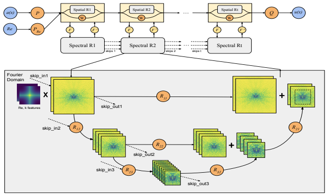
The load-bearing object is the scale-consistency identity (4), paired with sub-domain and super-domain sampling that turns it into a loss. Sub-domain sampling restricts input coefficient, boundary, and solution to a random patch, rescales the patch to unit size at the same grid resolution, and penalizes the difference between the model output on the patch and the restricted solution; super-domain sampling does the same when no ground-truth output is available, using the model's own prediction as the reference. The scale-informed neural operator backs this up by embedding the scale parameter (Reynolds number, wavenumber, viscosity) into Fourier-space features so the same network can represent very different frequencies. The theorem's proof machinery is an overlapping partition of unity: on each small subdomain the coefficient is nearly constant, exactness there plus scale consistency forces the operator to be a weak solution on each patch, and summing the weak forms over the partition yields the global solution.
What would settle it
A concrete check: train a neural operator with the scale-consistency loss on nearly constant coefficient data, measure the three terms in Theorem B.2, and evaluate on far-from-constant test fields; if a model achieves near-zero supervised, boundary, and consistency errors yet still shows large out-of-distribution error, the theorem's conclusion fails. Experimentally, one can also directly test whether the left and right sides of identity (4) agree to machine precision on all sampled subdomains for a trained model; if not, the model is in the regime the quantitative bound already leaves uncontrolled.
Extended reading notes
Core claim
The paper's core discovery is a self-supervised regularization scheme built on the exact scale-consistency identity (4): for an elliptic PDE, $T_\lambda G(a,g)$ restricted to the unit domain equals $G(T_\lambda a, T_\lambda G(a,g)|_{\partial\Omega})$. The authors prove Theorem 3.1 and its quantitative version Theorem B.2, showing that any operator satisfying this identity and matching the true solution operator on nearly constant coefficient fields must coincide with the true operator everywhere, with a bound expressing out-of-distribution error as the sum of supervised error, boundary error, and self-consistency error. Empirically, adding this loss to a scale-informed neural operator (an FNO with scale parameters embedded in Fourier space and a U-shaped multiband architecture) yields zero-shot extrapolation across scales: a 34% average error reduction across Burgers, Darcy, Helmholtz, and Navier-Stokes, including training at Re=1000 and testing at Re from 250 to 10,000.
Load-bearing premise
The load-bearing premise is that the system being modeled is governed by the same family of PDEs across all scales, so that rescaling a subdomain produces a valid instance of the same learned problem; the theorem also assumes the trained operator is exactly scale-consistent, exactly boundary-matching, and exactly correct on nearly constant coefficient fields, while training only minimizes those errors.
Editorial extensions
If this is right
- A model trained with scale-consistency at one scale parameter can be zero-shot evaluated at unseen scales; the paper reports Re 250–10,000 from Re 1000 training, and viscosity or wavenumber ranges beyond training.
- Scale-consistency is a self-supervised term: it requires only samples of inputs, not labeled solutions, so it can augment datasets where high-fidelity solution data is scarce.
- The quantitative bound in Theorem B.2 ties out-of-distribution error to three measurable quantities, giving a concrete regularization objective: reduce supervised error, boundary error, and consistency error separately.
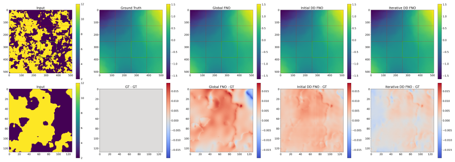
- Test-time domain decomposition with the pre-trained operator further reduces Darcy flow error by about 40% by iteratively refining local patches with informed boundary initialization.
- The architecture itself, with scale embedding plus a multiband U-shape, contributes to accuracy and parameter efficiency, matching FNO accuracy with roughly one tenth of the parameters in the cost-accuracy study.
Reading between the lines
- An implication the paper leaves implicit is that scale-consistency turns the scale parameter into a continuous dial: the same checkpoint could serve as the initialization for fine-tuning on a newly observed scale, potentially reducing data requirements for each new operating condition.
- Because the consistency identity applies even to PDEs like Helmholtz with no exact scale symmetry (after rescaling the wavenumber), the same machinery may extend to other parameter families, such as material contrasts or forcing frequencies, whenever the parameter transformation under rescaling is known.
- A testable extension is to measure the three error terms in Theorem B.2 during training and track whether out-of-distribution error tracks their sum; if the bound is tight in practice, it gives a model-selection criterion for when to trust a scale extrapolation.
Signed reviews
Editorial analysis
A structured set of objections, weighed in public.
Referee Report
Summary. This paper proposes a scale-consistency framework for training neural operators that can generalize across PDE scales. The authors define a scale-consistency loss based on PDE rescaling and sub-domain/super-domain sampling, provide a theorem claiming that scale consistency plus accuracy on nearly constant coefficient fields recovers the true solution operator (Theorems 3.1 and B.2), and introduce a scale-informed Fourier neural operator (SINO) with frequency embedding and a U-shaped multi-band structure. Experiments on Darcy flow, Burgers, Helmholtz, and Navier-Stokes report zero-shot generalization to unseen scales and a test-time domain-decomposition refinement that reduces Darcy error by about 40%.
Significance. If the theoretical and empirical claims hold, the work is a meaningful step toward scale-robust operator learning: the quantitative bound in Theorem B.2 is a genuine attempt to connect self-consistency to out-of-distribution error, and the proposed dataset and architecture address a real limitation of fixed-scale neural PDE solvers. The empirical direction is well motivated and, for the proposed SINO model, the improvements are consistent and sometimes large, for example on Burgers and Helmholtz. However, the advertised 'provable' statement is weaker than presented, and the experiments do not verify the quantities that appear in the theorem; moreover, several baseline comparisons show that scale-consistency can hurt. These issues currently prevent me from endorsing the central claims as stated.
major comments (3)
- [Section 3.1, Theorem 3.1; Appendix B.2, Theorem B.1] The theorem as stated in the main text claims that scale-consistency (4) plus accuracy on nearly constant coefficient functions implies Ψ ≡ G. The proof in Appendix B.2, Theorem B.1, requires two additional conditions: translation symmetry and exact boundary satisfaction (conditions 2 and 3 of Theorem B.1). The main text does not state these hypotheses, so the formal result is overstated. Please either state the full hypotheses in Theorem 3.1 or label it as an informal summary that points to the precise Theorem B.2.
- [Section 3.2.1, Algorithm 2; Section B.3, Theorem B.2] The super-domain loss is self-referential: Algorithm 2 penalizes mismatch between Ψ(a|Ω̂, Ψ(a,g,λk)|∂Ω̂, k) and Ψ(a,g,λk)|Ω̂, both of which use the model's own outputs as targets. An operator that outputs zero on the relevant inputs can satisfy this term exactly, so minimizing the training loss does not by itself tie Ψ to G. Theorem B.2 bounds Err_DM in terms of Err_Dδ, Err_boundary, and Err_selfcon, but the experiments neither measure these three sup-errors nor verify that the trained network is approximately scale-consistent, boundary-matching, and accurate on all of Dδ; training on a finite dataset with a weighted loss cannot establish the sup-error hypotheses. As a result, the theoretical guarantee is not connected to the empirical results. Please report these error quantities on validation sets or adapt the theorem to finite-sample or average errors with explicit assumptions.
- [Tables 1 and 2] The empirical claim that scale-consistency helps each model extrapolate is not consistently supported. For Burgers, UNO+scale is worse than UNO at the unseen ν=1/1000 (8.720 vs 8.624) and at the training ν=1/400 (1.387 vs 1.235), while UNet+scale is worse both in training and at ν=1/1000 (30.747 vs 26.481). For Navier-Stokes, UNet+scale deteriorates dramatically at the training Re=1000 (13.802 vs 0.809) and at Re=2000. The '34% average reduction' in the abstract needs to specify the aggregation across models and scales and should be accompanied by multiple seeds, error bars, and a discussion of cases where the method hurts.
minor comments (5)
- [Section 2, Related Work] There is a typo: 'scale consistenct framework' should be 'scale-consistency framework'.
- [Appendix D.1] The sentence 'As shown in Table 6, a minimum resolution of 32 per each dimension of space and time works the best' refers to a table that does not clearly present the minimum-size ablation; Table 6 reports the 2+1 dimensional Navier-Stokes results and has an unclear 'Aug. size min' column.
- [Equations (5)-(6) and Algorithms 1-2] Equation (6) and Algorithm 1 use ground-truth solutions, while Equation (5) and Algorithm 2 are self-supervised; the paper should distinguish the supervised sub-domain loss from the self-supervised super-domain loss more clearly, since both are called scale-consistency loss.
- [Figure 5] The caption uses 'RE=5000' while the text uses Re=5000; please unify the notation.
- [Abstract and Section 5] The claimed '34% error reduction on average of all datasets' is not directly traceable to a single table or aggregation rule; please define the average and identify which models and scales are included.
Circularity Check
Super-domain scale-consistency target is the model's own output; Theorem B.2's hypotheses are not shown to hold in training, so the regularizer reduces to a self-consistency condition rather than a constraint tying the model to the true operator.
-
self definitional
[Section 3.2.1, Algorithm 2 (lines 4-7), with Eq. (5)]
"estimate the solution of new domain u = Ψ(a,g,λk ). ... output: scale-consistency loss ∥Ψ(a|ˆΩ, Ψ(a,g,λk )|∂ ˆΩ,k )− Ψ(a,g,λk )|ˆΩ∥."
In Algorithm 2 the large-scale target is defined as the model's own output u = Ψ(a,g,λk). So the loss compares Ψ on a restricted input to a restriction of Ψ's own output. A zero operator (or any fixed point of the restriction map) satisfies this term exactly without approximating the true G. Theorem B.2 rescues the ideal case only when Err_Dδ(Ψ) and Err_boundary(Ψ) are small in sup-norm over near-constant inputs; the training minimizes a finite weighted loss and the paper never reports these sup-errors. Hence this unsupervised term is, by construction, a self-consistency condition on Ψ rather than a constraint tying Ψ to G, so the 'provable' recovery claim is not connected to the trained objective.
full rationale
The formal result Theorem 3.1/B.2 is not circular: it is a self-contained proof that an operator satisfying the exact scale-consistency identity (4), exact near-constant accuracy, and exact boundary matching must equal G. The zero-shot evaluations are performed against externally generated ground-truth solutions at scales not used in training, so those empirical claims do not reduce to fitted parameters. The circularity is confined to the super-domain sampling loss (Algorithm 2/Eq. (5)): its large-scale target is the model's own prediction, so that term is a fixed-point/equivariance constraint that degenerate operators satisfy identically. Because the paper does not verify the sup-norm quantities required by Theorem B.2, the theoretical guarantee is not established for the trained models. This is partial circularity in the self-supervised component, while the theorem's proof and the external benchmarks retain independent content; hence a score of 4 rather than 0 or 8.
Assumptions & free parameters
free parameters (1)
- Minimum sub-domain size for sub-sampling =
32 pixels
assumptions (3)
- domain assumption The elliptic PDE (Darcy flow) is well-posed: the coefficient a is uniformly coercive and the boundary data g is bounded, ensuring the solution operator G is unique and depends continuously on boundary data.
- ad hoc to paper The physics at all scales of interest is governed by the same family of PDEs with rescaled parameters; micro-scale physics is not described by a different model.
- ad hoc to paper The trained neural operator Ψ is close enough to the ideal conditions of Theorem B.2: exact or near-exact scale-consistency, exact boundary matching, and accuracy on nearly constant coefficient fields.
Cite this review
Pith. "Pith review of Scale-Consistent Learning for Partial Differential Equations." pith.science (2026). https://pith.science/paper/75USLMZV
@misc{pith2026250718813,
  author       = {Pith},
  title        = {Pith review of: Scale-Consistent Learning for Partial Differential Equations},
  year         = {2026},
  howpublished = {\url{https://pith.science/paper/75USLMZV}},
  note         = {Machine review of arXiv:2507.18813}
}
abstract
Machine learning (ML) models have emerged as a promising approach for solving partial differential equations (PDEs) in science and engineering. Previous ML models typically cannot generalize outside the training data; for example, a trained ML model for the Navier-Stokes equations only works for a fixed Reynolds number ($Re$) on a pre-defined domain. To overcome these limitations, we propose a data augmentation scheme based on scale-consistency properties of PDEs and design a scale-informed neural operator that can model a wide range of scales. Our formulation leverages the facts: (i) PDEs can be rescaled, or more concretely, a given domain can be re-scaled to unit size, and the parameters and the boundary conditions of the PDE can be appropriately adjusted to represent the original solution, and (ii) the solution operators on a given domain are consistent on the sub-domains. We leverage these facts to create a scale-consistency loss that encourages matching the solutions evaluated on a given domain and the solution obtained on its sub-domain from the rescaled PDE. Since neural operators can fit to multiple scales and resolutions, they are the natural choice for incorporating scale-consistency loss during training of neural PDE solvers. We experiment with scale-consistency loss and the scale-informed neural operator model on the Burgers' equation, Darcy Flow, Helmholtz equation, and Navier-Stokes equations. With scale-consistency, the model trained on $Re$ of 1000 can generalize to $Re$ ranging from 250 to 10000, and reduces the error by 34% on average of all datasets compared to baselines.
Figures


Figures from the paper (5 more)


Reference graph
Works this paper leans on
-
[1]
Kamyar Azizzadenesheli, Nikola Kovachki, Zongyi Li, Miguel Liu-Schiaffini, Jean Kossaifi, and Anima Anandkumar. Neural operators for accelerating scientific simulations and design.Nature Reviews Physics, pages 1–9, 2024
work page 2024
-
[2]
Jaideep Pathak, Shashank Subramanian, Peter Harrington, Sanjeev Raja, Ashesh Chattopadhyay, Morteza Mardani, Thorsten Kurth, David Hall, Zongyi Li, Kamyar Azizzadenesheli, et al. Fourcastnet: A global data-driven high-resolution weather model using adaptive fourier neural operators.arXiv preprint arXiv:2202.11214, 2022
arXiv 2022
-
[3]
Fourier neural operator for plasma modelling.arXiv preprint arXiv:2302.06542, 2023
Vignesh Gopakumar, Stanislas Pamela, Lorenzo Zanisi, Zongyi Li, Anima Anandkumar, and MAST Team. Fourier neural operator for plasma modelling.arXiv preprint arXiv:2302.06542, 2023
arXiv 2023
-
[4]
Neural operator: Graph kernel network for partial differential equations
Zongyi Li, Nikola Kovachki, Kamyar Azizzadenesheli, Burigede Liu, Kaushik Bhattacharya, Andrew Stuart, and Anima Anandkumar. Neural operator: Graph kernel network for partial differential equations. arXiv preprint arXiv:2003.03485, 2020
arXiv 2003
-
[5]
Neural operator: Learning maps between function spaces with applications to pdes.J
Nikola B Kovachki, Zongyi Li, Burigede Liu, Kamyar Azizzadenesheli, Kaushik Bhattacharya, Andrew M Stuart, and Anima Anandkumar. Neural operator: Learning maps between function spaces with applications to pdes.J. Mach. Learn. Res., 24(89):1–97, 2023
work page 2023
-
[6]
Lu Lu, Pengzhan Jin, Guofei Pang, Zhongqiang Zhang, and George Em Karniadakis. Learning nonlinear operators via DeepONet based on the universal approximation theorem of operators.Nature Machine Intelligence, 3(3):218–229, mar 2021
work page 2021
-
[7]
Learning operators with coupled attention.Journal of Machine Learning Research, 23(215):1–63, 2022
Georgios Kissas, Jacob H Seidman, Leonardo Ferreira Guilhoto, Victor M Preciado, George J Pappas, and Paris Perdikaris. Learning operators with coupled attention.Journal of Machine Learning Research, 23(215):1–63, 2022
work page 2022
-
[8]
Convolutional neural operators
Bogdan Raonic, Roberto Molinaro, Tobias Rohner, Siddhartha Mishra, and Emmanuel de Bezenac. Convolutional neural operators. InICLR 2023 Workshop on Physics for Machine Learning, 2023
2023
Show all 47 references
-
[9]
Fourier neural operator for parametric partial differential equations
Zongyi Li, Nikola Kovachki, Kamyar Azizzadenesheli, Burigede Liu, Kaushik Bhattacharya, Andrew Stuart, and Anima Anandkumar. Fourier neural operator for parametric partial differential equations. arXiv preprint arXiv:2010.08895, 2020. 15
2010 arXiv
-
[10]
Adaptive fourier neural operators: Efficient token mixers for transformers
John Guibas, Morteza Mardani, Zongyi Li, Andrew Tao, Anima Anandkumar, and Bryan Catan- zaro. Adaptive fourier neural operators: Efficient token mixers for transformers. arXiv preprint arXiv:2111.13587, 2021
2021 arXiv
-
[11]
U-no: U-shaped neural operators
Md Ashiqur Rahman, Zachary E Ross, and Kamyar Azizzadenesheli. U-no: U-shaped neural operators. arXiv preprint arXiv:2204.11127, 2022
2022 arXiv
-
[12]
Physics-informed neural operator for learning partial differential equations
Zongyi Li, Hongkai Zheng, Nikola Kovachki, David Jin, Haoxuan Chen, Burigede Liu, Kamyar Aziz- zadenesheli, and Anima Anandkumar. Physics-informed neural operator for learning partial differential equations. ACM/JMS Journal of Data Science, 2021
2021
-
[13]
Incorporating symmetry into deep dynamics models for improved generalization.arXiv preprint arXiv:2002.03061, 2020
Rui Wang, Robin Walters, and Rose Yu. Incorporating symmetry into deep dynamics models for improved generalization.arXiv preprint arXiv:2002.03061, 2020
2002 arXiv
-
[14]
Lie point symmetry data augmentation for neural pde solvers
Johannes Brandstetter, Max Welling, and Daniel E Worrall. Lie point symmetry data augmentation for neural pde solvers. InInternational Conference on Machine Learning, pages 2241–2256. PMLR, 2022
2022
-
[15]
Self-supervised learning with lie symmetries for partial differential equations
Grégoire Mialon, Quentin Garrido, Hannah Lawrence, Danyal Rehman, Yann LeCun, and Bobak Kiani. Self-supervised learning with lie symmetries for partial differential equations. Advances in Neural Information Processing Systems, 36:28973–29004, 2023
2023
-
[16]
Geometry-informed neural operator for large-scale 3d pdes.arXiv preprint arXiv:2309.00583, 2023
Zongyi Li, Nikola Borislavov Kovachki, Chris Choy, Boyi Li, Jean Kossaifi, Shourya Prakash Otta, Mo- hammad Amin Nabian, Christian Hundt Maximilian Stadler, Kamyar Azizzadenesheli, and Anima Anand- kumar. Geometry-informed neural operator for large-scale 3d pdes.arXiv preprint...
2023 arXiv
-
[17]
Ai-aided geometric design of anti-infection catheters
Tingtao Zhou, Xuan Wan, Daniel Zhengyu Huang, Zongyi Li, Zhiwei Peng, Anima Anandkumar, John F Brady, Paul W Sternberg, and Chiara Daraio. Ai-aided geometric design of anti-infection catheters. arXiv preprint arXiv:2304.14554, 2023
2023 arXiv
-
[18]
Scientific discovery in the age of artificial intelligence
Hanchen Wang, Tianfan Fu, Yuanqi Du, Wenhao Gao, Kexin Huang, Ziming Liu, Payal Chandak, Shengchao Liu, Peter Van Katwyk, Andreea Deac, et al. Scientific discovery in the age of artificial intelligence. Nature, 620(7972):47–60, 2023
2023
-
[19]
Pdebench: An extensive benchmark for scientific machine learning
Makoto Takamoto, Timothy Praditia, Raphael Leiteritz, Daniel MacKinlay, Francesco Alesiani, Dirk Pflüger, and Mathias Niepert. Pdebench: An extensive benchmark for scientific machine learning. Advances in Neural Information Processing Systems, 35:1596–1611, 2022
2022
-
[20]
Towards foundation models for scientific machine learning: Characterizing scaling and transfer behavior.Advances in Neural Information Processing Systems, 36, 2024
Shashank Subramanian, Peter Harrington, Kurt Keutzer, Wahid Bhimji, Dmitriy Morozov, Michael W Mahoney, and Amir Gholami. Towards foundation models for scientific machine learning: Characterizing scaling and transfer behavior.Advances in Neural Information Processing Systems, 36, 2024
2024
-
[21]
Multiple physics pretraining for physical surrogate models.arXiv preprint arXiv:2310.02994, 2023
Michael McCabe, Bruno Régaldo-Saint Blancard, Liam Holden Parker, Ruben Ohana, Miles Cranmer, Alberto Bietti, Michael Eickenberg, Siavash Golkar, Geraud Krawezik, Francois Lanusse, et al. Multiple physics pretraining for physical surrogate models.arXiv preprint arXiv:2310.02994, 2023
-
[22]
Dpot: Auto-regressive denoising operator transformer for large-scale pde pre-training
Zhongkai Hao, Chang Su, Songming Liu, Julius Berner, Chengyang Ying, Hang Su, Anima Anandkumar, Jian Song, and Jun Zhu. Dpot: Auto-regressive denoising operator transformer for large-scale pde pre-training. arXiv preprint arXiv:2403.03542, 2024
2024 arXiv
-
[23]
Ups: Towards foundation models for pde solving via cross-modal adaptation.arXiv preprint arXiv:2403.07187, 2024
Junhong Shen, Tanya Marwah, and Ameet Talwalkar. Ups: Towards foundation models for pde solving via cross-modal adaptation.arXiv preprint arXiv:2403.07187, 2024
2024 arXiv
-
[24]
Pretraining codomain attention neural operators for solving multiphysics pdes.arXiv preprint arXiv:2403.12553, 2024
Md Ashiqur Rahman, Robert Joseph George, Mogab Elleithy, Daniel Leibovici, Zongyi Li, Boris Bonev, Colin White, Julius Berner, Raymond A Yeh, Jean Kossaifi, et al. Pretraining codomain attention neural operators for solving multiphysics pdes.arXiv preprint arXiv:2403.12553, 2024
2024 arXiv
-
[25]
Springer Science & Business Media, 2008
Grigorios A Pavliotis and Andrew Stuart.Multiscale methods: averaging and homogenization, volume 53. Springer Science & Business Media, 2008. 16
2008
-
[26]
Learning homogenization for elliptic operators.SIAM Journal on Numerical Analysis, 62(4):1844–1873, 2024
Kaushik Bhattacharya, Nikola B Kovachki, Aakila Rajan, Andrew M Stuart, and Margaret Trautner. Learning homogenization for elliptic operators.SIAM Journal on Numerical Analysis, 62(4):1844–1873, 2024
2024
-
[27]
Domain decomposition methods for partial differential equations
Barry F Smith. Domain decomposition methods for partial differential equations. InParallel Numerical Algorithms, pages 225–243. Springer, 1997
1997
-
[28]
Exponential convergence for multiscale linear elliptic pdes via adaptive edge basis functions.Multiscale Modeling & Simulation, 19(2):980–1010, 2021
Yifan Chen, Thomas Y Hou, and Yixuan Wang. Exponential convergence for multiscale linear elliptic pdes via adaptive edge basis functions.Multiscale Modeling & Simulation, 19(2):980–1010, 2021
2021
-
[29]
Extended physics-informed neural networks (xpinns): A generalized space-time domain decomposition based deep learning framework for nonlinear partial differential equations
Ameya D Jagtap and George Em Karniadakis. Extended physics-informed neural networks (xpinns): A generalized space-time domain decomposition based deep learning framework for nonlinear partial differential equations. Communications in Computational Physics, 28(5), 2020
2020
-
[30]
Mosaic flows: A transferable deep learning framework for solving pdes on unseen domains.Computer Methods in Applied Mechanics and Engineering, 389:114424, 2022
Hengjie Wang, Robert Planas, Aparna Chandramowlishwaran, and Ramin Bostanabad. Mosaic flows: A transferable deep learning framework for solving pdes on unseen domains.Computer Methods in Applied Mechanics and Engineering, 389:114424, 2022
2022
-
[31]
Operator learning with domain decomposition for geometry generalization in pde solving.arXiv preprint arXiv:2504.00510, 2025
Jianing Huang, Kaixuan Zhang, Youjia Wu, and Ze Cheng. Operator learning with domain decomposition for geometry generalization in pde solving.arXiv preprint arXiv:2504.00510, 2025
2025
-
[32]
Spectral neural operators.arXiv preprint arXiv:2205.10573, 2022
Vladimir Fanaskov and Ivan Oseledets. Spectral neural operators.arXiv preprint arXiv:2205.10573, 2022
2022 arXiv
-
[33]
U-net: Convolutional networks for biomedical image segmentation
Olaf Ronneberger, Philipp Fischer, and Thomas Brox. U-net: Convolutional networks for biomedical image segmentation. InMedical Image Computing and Computer-Assisted Intervention–MICCAI 2015: 18th International Conference, Munich, Germany, October 5-9, 2015, Proceedings, Part I...
2015
-
[34]
Multiwavelet-based operator learning for differential equations
Gaurav Gupta, Xiongye Xiao, and Paul Bogdan. Multiwavelet-based operator learning for differential equations. Advances in neural information processing systems, 34:24048–24062, 2021
2021
-
[35]
Learning chaotic dynamics in dissipative systems
Zongyi Li, Miguel Liu-Schiaffini, Nikola Kovachki, Kamyar Azizzadenesheli, Burigede Liu, Kaushik Bhattacharya, Andrew Stuart, and Anima Anandkumar. Learning chaotic dynamics in dissipative systems. Advances in Neural Information Processing Systems, 35:16768–16781, 2022
2022
-
[36]
Towards multi-spatiotemporal-scale generalized pde modeling
Jayesh K Gupta and Johannes Brandstetter. Towards multi-spatiotemporal-scale generalized pde modeling. arXiv preprint arXiv:2209.15616, 2022
2022 arXiv
-
[37]
Score-based diffusion models in function space.arXiv preprint arXiv:2302.07400, 2023
Jae Hyun Lim, Nikola B Kovachki, Ricardo Baptista, Christopher Beckham, Kamyar Azizzadenesheli, Jean Kossaifi, Vikram Voleti, Jiaming Song, Karsten Kreis, Jan Kautz, et al. Score-based diffusion models in function space.arXiv preprint arXiv:2302.07400, 2023
2023 arXiv
-
[38]
Exponentially convergent multiscale methods for 2d high frequency heterogeneous helmholtz equations.Multiscale Modeling & Simulation, 21(3):849–883, 2023
Yifan Chen, Thomas Y Hou, and Yixuan Wang. Exponentially convergent multiscale methods for 2d high frequency heterogeneous helmholtz equations.Multiscale Modeling & Simulation, 21(3):849–883, 2023
2023
-
[39]
The cost-accuracy trade-off in operator learning with neural networks.arXiv preprint arXiv:2203.13181, 2022
Maarten V de Hoop, Daniel Zhengyu Huang, Elizabeth Qian, and Andrew M Stuart. The cost-accuracy trade-off in operator learning with neural networks.arXiv preprint arXiv:2203.13181, 2022
2022 arXiv
-
[40]
Deep complex networks
Chiheb Trabelsi, Olexa Bilaniuk, Ying Zhang, Dmitriy Serdyuk, Sandeep Subramanian, Joao Felipe Santos, Soroush Mehri, Negar Rostamzadeh, Yoshua Bengio, and Christopher J Pal. Deep complex networks. arXiv preprint arXiv:1705.09792, 2017
2017 arXiv
-
[41]
Spfno: Spectral operator learning for pdes with dirichlet and neumann boundary conditions.arXiv preprint arXiv:2312.06980, 2023
Ziyuan Liu, Yuhang Wu, Daniel Zhengyu Huang, Hong Zhang, Xu Qian, and Songhe Song. Spfno: Spectral operator learning for pdes with dirichlet and neumann boundary conditions.arXiv preprint arXiv:2312.06980, 2023. 17 A Datasets A.1 Darcy Flow We use a finite element solver with ...
2023 arXiv
-
[42]
For almost constantsa, we have Ψ(a,g ) =G(a,g ),
-
[43]
Ψ satisfies (4) exactly along with translation symmetry,
-
[44]
then we must necessarily haveΨ≡G
Ψ satisfies the boundary condition exactly. then we must necessarily haveΨ≡G . For a fully rigorous version, we refer to Theorem B.2 in the next Section B.3, which contains quantitative estimates for the approximation errorΨ≈G , by decomposing it into(1) an error on the near-c...
-
[45]
the error on the training distribution ErrDδ(Ψ),
-
[46]
the boundary condition error Errboundary(Ψ),
-
[47]
The simplified version in the main text is obtained when assuming that the supervised and unsupervised contributions in (17) vanish, implying that alsoErrDM = 0, i.e
and the self-consistency error Errselfcon.(Ψ). The simplified version in the main text is obtained when assuming that the supervised and unsupervised contributions in (17) vanish, implying that alsoErrDM = 0, i.e. Ψ(a,g ) =G(a,g ) for all (a,g )∈D M. Before coming to the proof...
2000
Reviewed August 15, 2026 · model on record in the stance chip above.
Discussion (0). Continue with ORCID to comment.