REVIEW 3 major objections 3 minor 1 cited by
Efficient quantum state tomography with Chebyshev polynomials
T0 review · 3 major / 3 minor · reviewed 2026-08-05 · deepseek-v4-flash
Pith's one-line read This paper makes approximate tomography of function-encoding quantum states far cheaper by measuring only a truncated Chebyshev expansion, with measurement and post-processing costs that do not grow with qubit count.
desk verdict Clever spectral readout for states with known preparation circuits, but the 'tomography' framing overreaches and the shot-count scaling is wrong by a factor of ε. read the letter →
The pith
A machine-rendered reading of the paper's core claim, the machinery that carries it, and where it could break.
The reading
What carries the argument
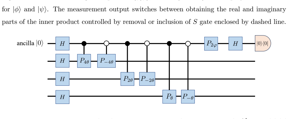
The load-bearing identity is $\langle T_{s,n} | \psi \rangle = \langle F, \tilde{T}_{s,2^n} \rangle_{2^n}$: the overlap between the target state and a Chebyshev basis state equals the discrete Chebyshev inner product, so every expansion coefficient becomes a circuit-measurable quantity. The basis state $|T_{s,n}\rangle$ is prepared by a quantum-Fourier-transform-style circuit whose $|0\rangle$ branch carries $\cos\left(\frac{(2k+1)s\pi}{2^{n+1}}\right)$ at position $k$, with overall 75% success probability; the Hadamard test with an optional S gate then reads the real and imaginary parts of the overlap. The discrete orthogonality of Chebyshev polynomials at their zeros supplies normalization, and the classical convergence bound for truncated Chebyshev series justifies
What would settle it
Run QST-CP on a state encoding a function whose Chebyshev coefficients decay slowly, for example $f(x)=\operatorname{sgn}(x)$ or a sinusoid whose frequency grows with n, at fixed threshold $A_c=0.9$ and increasing qubit count n. If achieving the threshold forces the stopping order m to grow with n, then the claimed n-independence of measurement repetitions fails outside scale-concentrated states; if m stays constant while fidelity remains high, the claim is universal.
Extended reading notes
Core claim
QST-CP reduces approximate tomography of a pure state encoding a continuous function to estimating Chebyshev expansion coefficients. Normalized Chebyshev basis states are constructed so that their inner product with the target equals the discrete Chebyshev coefficient; a Hadamard test with an optional S gate reads real and imaginary parts. The partial sum $A_m$ of squared coefficients tracks captured energy, and measurement stops once $A_m \geq A_c$. When energy concentrates in low-order modes, m stays small as n grows: measurement repetitions are $O\left(\frac{(4m/3)^d}{\epsilon d!}\right)$ and post-processing $O\left(\frac{m^d}{d!}\right)$, both independent of n, with linear-depth circuits. Analytic and turbulent-flow tests recover dominant l
Load-bearing premise
The load-bearing premise is that the target state has a known preparation unitary that can be controlled for the Hadamard test and that its encoded function concentrates its squared amplitude in low-order Chebyshev modes; if either condition fails, the coefficients either cannot be measured at all or the truncated reconstruction stops being faithful as n grows.
Editorial extensions
If this is right
- Measurement repetitions and post-processing do not grow with qubit count for function-encoding states whose energy is concentrated in low-order modes, directly removing the exponential bottleneck of full tomography in that setting.
- The stopping rule A_m ≥ A_c gives a built-in accuracy-efficiency tradeoff: lowering the threshold gives a cheaper coarse reconstruction, while raising it resolves finer scales.
- Circuit depth stays linear in n whenever the target state has a shallow preparation circuit, so the method is compatible with near-term hardware for moderate n.
- For d-dimensional functions the basis count grows like m^d/d!, so low-dimensional fields are practical; the (4/3)^d factor in repetition count penalizes high-dimensional cases.
- The method is tailored to large-scale feature recovery, so it can serve as a readout protocol for quantum PDE solvers whose outputs are smooth fields rather than a replacement for full tomography of arbitrary states.
Reading between the lines
- Extension: the practical reach of the protocol is states whose preparation circuit is known and controllable; for a genuinely unknown state the controlled preparation required by the Hadamard test is not available, so the 'tomography' label applies only in that narrower setting.
- Extension: the 75%-success basis preparation contributes the (4/3)^d factor; amplitude amplification on the basis-preparation ancilla would likely reduce this to a constant overhead, improving high-dimensional cases the paper does not explore.
- Extension: the same coefficient-estimation loop could be embedded as a readout head in variational or block-encoding solvers, with the solver's own ansatz supplying the controlled preparation unitary and A_m acting as a convergence monitor.
Editorial analysis
A structured set of objections, weighed in public.
Referee Report
Summary. The paper proposes QST-CP, an approximate tomography method for pure quantum states that encode continuous (possibly multivariate) complex-valued functions. The target state is expanded in a truncated Chebyshev basis; the expansion coefficients are obtained as inner products between the target state and Chebyshev-basis states, measured via a Hadamard test. The authors give a circuit for preparing the normalized Chebyshev basis states, a stopping criterion based on the cumulative coefficient energy A_m, and complexity claims stating that the number of measurement repetitions and the classical post-processing are independent of the qubit count n. Numerical simulations on analytic functions and on turbulent-flow data are used to validate the method.
Significance. If the central claims hold, the paper would offer a practical readout method for quantum states produced by known circuits, particularly in quantum computational fluid dynamics, where states encode smooth flow fields. The mathematical core is largely self-contained: the expansion coefficients are defined as discrete inner products and are directly measured, so the procedure is not circular in the sense of fitting parameters from the measured data. The manuscript also provides explicit circuits, a clear stopping criterion, reproducible code, and numerical demonstrations on realistic flow data. However, the protocol's dependence on a known and controllable state-preparation unitary is a major scope restriction, and the complexity analysis contains a shot-count error and an unclear post-processing claim. These issues affect the paper's central efficiency and tomography claims.
major comments (3)
- [Section III.A, Fig. 2] The Hadamard-test inner-product measurement requires a controlled version of U_psi for the target state. For a genuinely unknown state—the standard QST setting—U_psi is not available, and a swap test yields only |<psi|T_{s,n}>|^2, losing the sign/phase needed for the complex coefficients. Thus QST-CP is a readout protocol for states whose preparation circuit is known and controllable, not a general tomography method. The abstract and Section II.A compare to full measurement-based QST without flagging this restriction. Please state this limitation explicitly and temper the tomography framing, or provide a sign-recovery scheme that does not require U_psi.
- [Section III.C, Table I] The measurement-repetition count is underestimated by a power of epsilon. Estimating an inner product to precision epsilon with a Hadamard test requires O(1/epsilon^2) shots, not O(1/epsilon). Consequently the total repetition count should be O((4m/3)^d/(epsilon^2 d!)) for the multivariate case and O(4m/(3 epsilon^2)) for the single-variable case, not the expressions in the text and Table I. The qualitative n-independence survives, but the stated complexity is incorrect and must be corrected.
- [Section III.C, Table I] The post-processing claim is ambiguous and, as stated, inconsistent with reconstructing a quantum state. If the output is a reconstructed state vector of length 2^n, evaluating the truncated Chebyshev series at all grid points costs at least Omega(2^n) (or Omega(2^n m^d) depending on the evaluation method), so the post-processing cannot be O(1) or O(m^d/d!) independent of n. If the output is only the set of expansion coefficients or a single amplitude, that is not full state reconstruction. Please clarify what 'post-processing' computes and reconcile it with the tomography claim.
minor comments (3)
- [Eq. (5)] The discrete orthogonality relation is stated for 0 <= s,t <= p, but for s=t=p the sum is zero because T_p vanishes at its own zeros. The correct statement is for 0 <= s,t < p. Since the expansions use P <= p-1, this does not affect the main results, but the displayed equation is formally false.
- [Eq. (12)] The notation is inconsistent: the subscript list is written as (s_1,...,s_n,n_1,...,n_d) and (s_1,...,s_n) in the summation in Eq. (13). The number of variables is d, not n. Please correct the subscripting.
- [Section IV.A] All numerical results use only 500 measurement repetitions per coefficient. The visible deviations in Figs. 6(b,d) are attributed to sampling error; a brief note on the expected amplitude of statistical fluctuations at 500 shots would help the reader interpret the fidelity numbers.
Circularity Check
No significant circularity: QST-CP measures Chebyshev coefficients directly via inner products and reconstructs from them without fitted-input redirection.
full rationale
The derivation is self-contained. Equation (9) defines the Chebyshev basis states; Eq. (5) gives the discrete orthogonality relation; Eq. (10) and Fig. 3 show how to prepare them; and the Hadamard-test circuit of Fig. 2 measures Re/Im of ⟨T_s,n|ψ⟩, which by Eq. (8) is exactly the expansion coefficient a_s. Reconstruction is just the truncated Chebyshev series using the measured coefficients. No parameter is fitted to a subset of data and then presented as a prediction of closely related data; the stopping criterion A_m in Eq. (11) is an adaptive rule based on measured coefficients, not a source of the reconstructed amplitudes. The complexity claims in Section III.C follow from circuit depth and repetition counting, not from any fitted quantity. The paper contains self-citations (e.g., refs. [5], [10], [18], [19], [25], [43]), but these are contextual or code-availability citations and are not load-bearing for the central mathematical derivation. The main caveat—that the Hadamard test requires access to the controlled state-preparation unitary U_ψ (Section III.A)—is a scope restriction on the method's applicability to known, controllable state preparations, not a circular step; it concerns the framing as 'tomography' rather than the internal consistency of the derivation. No circular reduction is evident, so the appropriate score is 0.
Assumptions & free parameters
free parameters (3)
- Stopping threshold A_c =
0.85, 0.5, 0.9 (chosen per experiment)
- Truncation order m =
3, 7, 11, 19, 30, 60, 90 (in experiments)
- Number of measurement shots per coefficient =
500
assumptions (4)
- domain assumption The target quantum state is a pure state with amplitudes equal to function values on a grid (Eq. 1).
- domain assumption The function's Chebyshev spectrum decays fast enough that low-order truncation captures dominant energy.
- domain assumption The state preparation unitary U_psi is known and can be controlled.
- standard math Hadamard test measurements give unbiased estimates of inner products with standard sampling error.
Cite this review
Pith. "Pith review of Efficient quantum state tomography with Chebyshev polynomials." pith.science (2026). https://pith.science/paper/DUN2CTL4
@misc{pith2026250902112,
  author       = {Pith},
  title        = {Pith review of: Efficient quantum state tomography with Chebyshev polynomials},
  year         = {2026},
  howpublished = {\url{https://pith.science/paper/DUN2CTL4}},
  note         = {Machine review of arXiv:2509.02112}
}
read the original abstract
Quantum computing shows promise for addressing computationally intensive problems but is constrained by the exponential resource requirements of general quantum state tomography (QST), which fully characterizes quantum states through parameter estimation. We introduce the QST with Chebyshev polynomials, an approximate tomography method for pure quantum states encoding complex-valued functions. This method reformulates tomography as the estimation of Chebyshev expansion coefficients, expressed as inner products between the target quantum state and Chebyshev basis functions, measured using the Hadamard test circuit. By treating the truncation order of the Chebyshev polynomials as a controllable parameter, the method provides a practical balance between efficiency and accuracy. For quantum states encoding functions dominated by large-scale features, such as those representing fluid flow fields, appropriate truncation enables faithful reconstruction of the dominant components via quantum circuits with linear depth, while keeping both measurement repetitions and post-processing independent of qubit count, in contrast to the exponential scaling of full measurement-based QST methods. Validation on analytic functions and numerically generated flow-field data demonstrates accurate reconstruction and effective extraction of large-scale features, indicating the method's suitability for systems governed by macroscopic dynamics.
Figures


Figures from the paper (7 more)


Forward citations
Cited by 1 Pith paper
-
Quantum simulation of real-world nonlinear dynamics via Koopman method
A learned Koopman embedding plus shallow LCHS circuits simulates moderately nonlinear dynamics on NISQ hardware and marks the noise-to-representation performance boundary.
Reference graph
Works this paper leans on
-
[1]
M. A. Nielsen, I. L. Chuang, Quantum Computation and Quantum Information, Cambridge University Press, 2010
work page 2010
-
[2]
Wittek, Quantum machine learning: what quantum computing means to data mining, Academic Press, 2014
P. Wittek, Quantum machine learning: what quantum computing means to data mining, Academic Press, 2014
work page 2014
-
[3]
Y. Cao, J. Romero, J. P. Olson, M. Degroote, P. D. Johnson, M. Kieferov´ a, I. D. Kivlichan, T. Menke, B. Peropadre, N. P. D. Sawaya, et al., Quantum chemistry in the age of quantum computing, Chem. Rev. 119 (2019) 10856–10915
work page 2019
-
[4]
S. Jin, N. Liu, Y. Yu, Quantum simulation of partial differential equations: Applications and detailed analysis, Phys. Rev. A 108 (2023) 032603
work page 2023
-
[5]
Z. Meng, J. Zhong, S. Xu, K. Wang, J. Chen, F. Jin, X. Zhu, Y. Gao, Y. Wu, C. Zhang, N. Wang, Y. Zou, A. Zhang, Z. Cui, F. Shen, Z. Bao, Z. Zhu, Z. Tan, T. Li, P. Zhang, S. Xiong, H. Li, Q. Guo, Z. Wang, C. Song, H. Wang, Y. Yang, Simulating unsteady fluid flows on a superconducting quantum processor, Commun. Phys. 7 (2024) 349
work page 2024
-
[6]
Y. Xiao, L. M. Yang, C. Shu, S. C. Chew, B. C. Khoo, Y. D. Cui, Y. Y. Liu, Physics- informed quantum neural network for solving forward and inverse problems of partial dif- ferential equations, Phys. Fluids 36 (2024) 9
work page 2024
- [7]
-
[8]
S. S. Bharadwaj, K. R. Sreenivasan, Towards simulating fluid flows with quantum comput- ing, S¯ adhan¯ a 50 (2025) 1–19
work page 2025
Show all 49 references
-
[9]
Tennie, S
F. Tennie, S. Laizet, S. Lloyd, L. Magri, Quantum computing for nonlinear differential equations and turbulence, Nat. Rev. Phys. 7 (2025) 220–230
2025
-
[10]
Z. Y. Meng, C. Song, Y. Yang, Challenges of simulating fluid flows on near-term quantum computer, Sci. China-Phys. Mech. Astron. 68 (2025) 104705. 21
2025
-
[11]
Steijl, G
R. Steijl, G. N. Barakos, Parallel evaluation of quantum algorithms for computational fluid dynamics, Comput. Fluids 173 (2018) 22–28
2018
-
[12]
Gaitan, Finding flows of a Navier-Stokes fluid through quantum computing, NPJ Quantum Inf
F. Gaitan, Finding flows of a Navier-Stokes fluid through quantum computing, NPJ Quantum Inf. 6 (2020) 61
2020
-
[13]
Lubasch, J
M. Lubasch, J. Joo, P. Moinier, M. Kiffner, D. Jaksch, Variational quantum algorithms for nonlinear problems, Phys. Rev. A 101 (2020) 010301
2020
-
[14]
Gourianov, M
N. Gourianov, M. Lubasch, S. Dolgov, Q. Y. van den Berg, H. Babaee, P. Givi, M. Kiffner, D. Jaksch, A quantum-inspired approach to exploit turbulence structures, Nat. Comput. Sci. 2 (2022) 30–37
2022
-
[15]
Pfeffer, F
P. Pfeffer, F. Heyder, J. Schumacher, Hybrid quantum-classical reservoir computing of thermal convection flow, Phys. Rev. Res. 4 (2022) 033176
2022
-
[16]
Zylberman, G
J. Zylberman, G. D. Molfetta, M. Brachet, N. F. Loureiro, F. Debbasch, Quantum sim- ulations of hydrodynamics via the Madelung transformation, Phys. Rev. A 106 (2022) 032408
2022
-
[17]
Fukagata, Towards quantum computing of turbulence, Nat
K. Fukagata, Towards quantum computing of turbulence, Nat. Comput. Sci. 2 (2022) 68–69
2022
-
[18]
Z. Y. Meng, Y. Yang, Quantum computing of fluid dynamics using the hydrodynamic Schr¨ odinger equation, Phys. Rev. Research 5 (2023) 033182
2023
-
[19]
Z. Y. Meng, Y. Yang, Quantum spin representation for the Navier-Stokes equation, Phys. Rev. Research 6 (2024) 043130
2024
-
[20]
Jaksch, P
D. Jaksch, P. Givi, A. J. Daley, T. Rung, Variational quantum algorithms for computational fluid dynamics, AIAA J. 61 (2023) 1885–1894
2023
-
[21]
Y. Liu, Z. Chen, C. Shu, P. Rebentrost, Y. Liu, S. Chew, B. Khoo, Y. Cui, A variational quantum algorithm-based numerical method for solving potential and Stokes flows, Ocean Eng. 292 (2024) 116494
2024
-
[22]
Z. Y. Chen, T. Y. Ma, C. C. Ye, L. Xu, W. Bai, L. Zhou, M. Y. Tan, X. N. Zhuang, X. F. Xu, Y. J. Wang, Enabling large-scale and high-precision fluid simulations on near-term quantum computers, Comput. Methods Appl. Mech. Eng. 432 (2024) 117428
2024
-
[23]
S. S. Bharadwaj, K. R. Sreenivasan, Hybrid quantum algorithms for flow problems, Proc. Natl. Acad. Sci. 120 (2023) e2311014120
2023
-
[24]
Itani, K
W. Itani, K. R. Sreenivasan, S. Succi, Quantum algorithm for lattice Boltzmann (QALB) simulation of incompressible fluids with a nonlinear collision term, Phys. Fluids 36 (2024) 22 017112
2024
-
[25]
B. Y. Wang, Z. Y. Meng, Y. M. Zhao, Y. Yang, Quantum lattice Boltzmann method for simulating nonlinear fluid dynamics, arXiv:2502.16568 (2025)
2025 arXiv
-
[26]
Gross, Y
D. Gross, Y. K. Liu, S. T. Flammia, S. Becker, J. Eisert, Quantum state tomography via compressed sensing, Phys. Rev. Lett. 105 (2010) 150401
2010
-
[27]
C. A. Riofrio, D. Gross, S. T. Flammia, T. Monz, D. Nigg, R. Blatt, J. Eisert, Experimental quantum compressed sensing for a seven-qubit system, Nature Commun. 8 (2017) 15305
2017
-
[28]
Banaszek, G
K. Banaszek, G. M. D’ariano, M. G. A. Paris, M. F. Sacchi, Maximum-likelihood estimation of the density matrix, Phys. Rev. A 61 (1999) 010304
1999
-
[29]
J. W. Shang, Z. Y. Zhang, H. K. Ng, Superfast maximum-likelihood reconstruction for quantum tomography, Phys. Rev. A 95 (2017) 062336
2017
-
[30]
Ferrie, Self-guided quantum tomography, Phys
C. Ferrie, Self-guided quantum tomography, Phys. Rev. Lett. 113 (2014) 190404
2014
-
[31]
Bolduc, G
E. Bolduc, G. C. Knee, E. M. Gauger, J. Leach, Projected gradient descent algorithms for quantum state tomography, npj Quantum Information 3 (2017) 44
2017
-
[32]
Torlai, R
G. Torlai, R. G. Melko, Machine-learning quantum states in the NISQ era, Annu. Rev. Condens. Matter Phys. 11 (2020) 325–344
2020
-
[33]
Ahmed, M
S. Ahmed, M. C. Sanchez, F. Nori, A. F. Kockum, Quantum state tomography with conditional generative adversarial networks, Phys. Rev. Lett. 127 (2021) 140502
2021
-
[34]
Koutn` y, L
D. Koutn` y, L. Motka, Z. Hradil, J. ˇReh´ aˇ cek, L. L. S. Soto, Neural-network quantum state tomography, Phys. Rev. A 106 (2022) 012409
2022
-
[35]
H. Y. Huang, R. Kueng, J. Preskill, Predicting many properties of a quantum system from very few measurements, Nature Phys. 16 (2020) 1050–1057
2020
-
[36]
Cotler, F
J. Cotler, F. Wilczek, Quantum overlapping tomography, Phys. Rev. Lett. 124 (2020) 100401
2020
-
[37]
Y. Liu, D. Y. Wang, S. C. Xue, A. Q. Huang, X. Fu, X. G. Qiang, P. Xu, H. L. Huang, M. T. Deng, C. Guo, et al., Variational quantum circuits for quantum state tomography, Phys. Rev. A 101 (2020) 052316
2020
-
[38]
Steffens, C
A. Steffens, C. A. Riofr ´ ıo, W. McCutcheon, I. Roth, B. A. Bell, A. McMillan, M. S. Tame, J. G. Rarity, J. Eisert, Experimentally exploring compressed sensing quantum tomography, Quantum Sci. Technol. 2 (2017) 025005
2017
-
[39]
Cramer, M
M. Cramer, M. B. Plenio, S. T. Flammia, R. Somma, D. Gross, S. D. Bartlett, O. L. Cardinal, D. Poulin, Y. K. Liu, Efficient quantum state tomography, Nat. Commun. 1 23 (2010) 149
2010
-
[40]
B. P. Lanyon, C. Maier, M. Holz¨ apfel, T. Baumgratz, C. Hempel, P. Jurcevic, I. Dhand, A. S. Buyskikh, A. J. Daley, M. Cramer, et al., Efficient tomography of a quantum many- body system, Nature Phys. 13 (2017) 1158–1162
2017
-
[41]
Kyriienko, A
O. Kyriienko, A. E. Paine, V. E. Elfving, Solving nonlinear differential equations with differentiable quantum circuits, Phys. Rev. A 103 (2021) 052416
2021
-
[42]
Sarma, T
A. Sarma, T. W. Watts, M. Moosa, Y. Liu, P. L. McMahon, Quantum variational solving of nonlinear and multidimensional partial differential equations, Phys. Rev. A 109 (2024) 062616
2024
-
[43]
Codes available athttps://github.com/YYgroup/ChebyMeasure, 2025
2025
-
[44]
A. N. Kolmogorov, The local structure of turbulence in incompressible viscous fluid for very large Reynolds numbers, Dokl. Akad. Nauk SSSR 30 (1941) 301–305
1941
-
[45]
T. J. Rivlin, Chebyshev polynomials, Courier Dover Publications, 2020
2020
-
[46]
L. N. Trefethen, Approximation theory and approximation practice, extended edition, SIAM, 2019
2019
-
[47]
A. J. Abhari, M. Treinish, K. Krsulich, C. J. Wood, J. Lishman, J. Gacon, S. Martiel, P. D. Nation, L. S. Bishop, A. W. Cross, B. R. Johnson, J. M. Gambetta, Quantum computing with Qiskit, arXiv.2405.08810 (2024)
2024 arXiv
-
[48]
S. A. Orszag, Numerical methods for the simulation of turbulence, Phys. Fluids 12 (1969) II–250
1969
-
[49]
Graham, K
J. Graham, K. Kanov, X. I. A. Yang, M. K. Lee, N. Malaya, C. C. Lalescu, R. Burns, G. Eyink, A. Szalay, R. D. Moser, C. Meneveau, A web services accessible database of turbulent channel flow and its use for testing a new integral wall model for LES, Journal of Turbulence 17 (2...
2016
Reviewed August 5, 2026 · model on record in the stance chip above.
Discussion (0). Continue with ORCID to comment.