REVIEW 1 major objections 5 minor 31 references
Efficient and Robust Carath\'{e}odory-Steinitz Pruning of Positive Discrete Measures
T0 review · 1 major / 5 minor · reviewed 2026-08-04 · deepseek-v4-flash
Pith's one-line read This paper establishes that Carathéodory–Steinitz pruning can be run as a streaming algorithm with O(N^2) storage and O((M−N)N^2 + N^3) total work, and that the pruning map is locally Lipschitz with respect to total variation distance.
desk verdict Solid algorithmic contribution for Carathéodory–Steinitz pruning, but the stability theorem is proven with an exponentially small radius, so the numerical experiments do not actually probe it in the large-M regime. read the letter →
The pith
A machine-rendered reading of the paper's core claim, the machinery that carries it, and where it could break.
The reading
What carries the argument
The central object is the Vandermonde-like moment matrix V ∈ R^{M×N} whose columns are the N basis functions evaluated at the M nodes. CSP repeatedly finds a nonzero vector in the cokernel of V^T, moves the weight vector along that direction until one weight hits zero, and deletes that node. SCSP restricts the working set to N+k rows at a time, and GSCSP maintains a dense (N+k)×N QR factorization, with Givens-rotation downdates and updates to replace one row per iteration; the cokernel vector is a trailing column of Q, available in O(N^2) work per step.
What would settle it
For the complexity claim, time one full GSCSP run for fixed M and N = 8, 16, 32, 64 and fit the per-iteration cost; if it grows faster than O(N^2), the advertised per-step complexity is wrong. For the stability claim, run SCSP on a Chebyshev-system node set and perturb the weights by total-variation amounts of 10^-8, 10^-6, and 10^-4; if the output distance does not shrink proportionally, the Lipschitz conclusion of Theorem 4.1 is violated.
Extended reading notes
Core claim
The core discovery is the GSCSP algorithm: a streaming Carathéodory–Steinitz pruning in which the cokernel vector needed at each step is extracted from a maintained QR factorization of a small (N+1)×N window of the Vandermonde-like matrix, and the factorization is updated after each deletion and insertion using Givens rotations. This reduces per-iteration complexity from O(MN^2) to O(N^2) and storage from O(MN) to O(N^2). The paper also proves Theorem 4.1: under a Chebyshev-system assumption on the moment matrix, a fixed node ordering, and a unique minimizer of the sign-selection rule, the SCSP (hence GSCSP) output is locally Lipschitz with respect to total variation distance, so small admis
Load-bearing premise
For the stability half of the claim, the load-bearing premise is that every N-point subset of the nodes gives a nonsingular moment matrix (a Chebyshev system), together with a fixed node ordering and a unique argmin in the sign-selection step; if any N-by-N submatrix is singular, the cokernel vector is non-unique and the pruning path can jump under arbitrarily small perturbations.
Editorial extensions
If this is right
- A positive M-point rule with M ≫ N can be compressed to N points while exactly preserving N moments using storage that depends only on N, not M.
- Total runtime is O((M−N)N^2 + N^3), i.e., linear in M, making billion-point compression feasible with modest memory.
- Small total-variation perturbations that preserve the node ordering—including perturbations that add new nodes with small weights—change the pruned rule by at most a constant times the perturbation size (Theorem 4.1).
- The same pruning can be applied to non-polynomial spaces V, as long as the moment conditions are well-defined.
- The algorithm generates positive, moment-preserving quadrature on cut-cell geometries, directly usable in discontinuous Galerkin discretizations.
Reading between the lines
- Because the stability theorem is tied to a fixed ordering of the input nodes, a natural extension is a permutation-invariant or ordering-adaptive variant; the paper gives no such guarantee, and its own analysis shows reordering can change the output.
- The Chebyshev-system hypothesis fails for structured multivariate node sets (e.g., nodes on a line for monomial bases); a pivoting strategy or random shuffling of inputs might restore uniqueness generically, at the cost of a different stability statement.
- The Lipschitz constant in the proof grows geometrically through the sequence C_j, so the worst-case bound may be conservative; measuring actual output variation across perturbation scales would show whether practical stability is far better than the theorem guarantees.
- The O(N^2) storage opens the door to pruning in high-dimensional settings where N is large but M is astronomical, provided the moment matrix can be formed row-by-row; this is exactly the streaming regime the algorithm targets.
Editorial analysis
A structured set of objections, weighed in public.
Referee Report
Summary. The paper develops a streaming implementation of Carathéodory–Steinitz pruning for compressing a positive M-node quadrature measure to an N-node measure preserving N moments in a finite-dimensional space V. The SCSP algorithm (Alg. 2) retains only N+k rows of the Vandermonde-like matrix at a time, and the GSCSP variant (Alg. 3) uses Givens row downdates/updates so that each iteration costs O(N^2), giving total O((M-N)N^2+N^3) work and O(N^2) storage. Theorem 4.1 asserts local Lipschitz continuity in a normalized total-variation metric under admissible perturbations, assuming a Chebyshev-system condition, fixed ordering, k=1, and unique selection at every iteration. The numerical section compares GSCSP with NNLS and LP, demonstrates large-scale pruning, and includes a cut-cell discontinuous Galerkin application.
Significance. The algorithmic contribution is solid and practically relevant: for the M≫N regime, GSCSP removes the dominant storage bottleneck of naive CSP, and the Givens downdate/update mechanism is an appropriate and well-executed device. The paper provides clear pseudocode, a complexity analysis, a detailed proof of Theorem 4.1 in Appendix A, and reproducible open-source code in CaratheodoryPruning.jl. The stability theorem is a step toward understanding perturbation behavior of pruning algorithms, and the experiments usefully contrast GSCSP, NNLS, and LP. However, as detailed below, the quantitative stability guarantee is currently far too weak to justify the practical 'robust' claim in the advertised large-M regime, and the numerical stability experiments are not actually covered by Theorem 4.1. With an honest reframing of the stability claims, the paper would be acceptable.
major comments (1)
- [Section 4.2 / Appendix A, Eq. (21) and the definition of δ2] The stability theorem is stated as a quantitative Lipschitz bound, but its constants are exponential in M-N and the admissible radius is astronomically small in the paper's own target regime. From C_j=(1+N_j)C_{j-1}+1 and N_j≥1, one gets C_{M-N}≥2^{M-N+1}-1; in the Figure 5 example M=10^4, N=113, so C_{M-N}≳2^{9888}≈10^{2977}. Consequently δ2 ≤ (1/(3|µM|)) min_j ϵ_j/C_j is below ~10^{-2977} even if every ϵ_j were of order 1, and the Lipschitz constant C in the theorem contains the same exponential factor. The perturbations tested in Figure 5 begin at d_TV=10^{-10}, so every plotted point lies outside the radius for which the bound is proven. Therefore the statement in Section 5.3 that these experiments provide 'supporting evidence' for the TV-stability theorem is not justified. The theorem may be true, but it currently establishes only qualitative continuity, not practical robustness in
minor comments (5)
- [Table 1] The complexity entry for SCSP appears inconsistent with Section 3.1. The table lists per-iteration complexity M N^2 for SCSP, but the text states that fixed-k SCSP computes a cokernel vector of an (N+k)×N matrix at cost O(N^3) per iteration and O((M-N)N^3) total. If the table is per-iteration, the entry should be N^3; if it is cumulative, the CSP and SCSP entries need to be adjusted accordingly.
- [Section 5.3] Please temper the language that the numerical stability tests 'support' Theorem 4.1. Since the tested perturbations are many orders of magnitude larger than the proven δ0, the experiments should be described as empirical stability observations in a regime not covered by the theorem, rather than as confirmation of the theorem.
- [Algorithm 3] The output line 'k ← M∗{N+1}' appears garbled; presumably it should be 'n ← Q_{*,N+1}' or similar. As printed, it is not readable pseudocode.
- [Section 4, intro] The sentence 'This result immediately applies to the GSCSP algorithm' should be qualified: the theorem is proved for the exact SCSP procedure in exact arithmetic. The floating-point Givens updates in GSCSP introduce roundoff, and no roundoff analysis is supplied, so the formal stability guarantee does not automatically transfer to the implemented floating-point algorithm.
- [Section 5.2.2] There is a typo: 'Figure Figure 6' should read 'Figure 6'.
Circularity Check
No significant circularity: GSCSP complexity and SCSP stability are independently derived from explicit algorithms and adjoint perturbation tracking.
full rationale
The paper's central derivation chain is not circular. The SCSP/GSCSP algorithms are explicit, executable procedures (Algorithms 2 and 3), and the claimed O(N^2) storage and O((M-N)N^2 + N^3) complexity are operation counts built from the Givens downdate/update procedure, which is an external standard result [14]; no fitted parameter is later relabeled as a prediction. Theorem 4.1's local-Lipschitz claim is also not assumed in its inputs: Assumption 4.1 and Definition 4.1 only pin down a unique unperturbed pruning path, while Appendix A independently constructs delta0 and C from the optimality gaps epsilon_j, normalized kernel masses N_j, the matrix U, and the weight margin u, then proves by induction that a sufficiently small admissible perturbation leaves the pruning choices unchanged. That is a genuine proof, not a renaming or an imported uniqueness theorem. The self-citations in the manuscript ([5], [21], [23], [24]) are used for applications and context (entropy-stable DG, reduced-order modeling, cut-cell quadrature construction), not as evidence for the new stability bound or complexity estimate. The numerical sections compare GSCSP against external NNLS and LP implementations; the stability experiments are supporting examples rather than the proof. The most serious weakness is that Theorem 4.1's guaranteed perturbation radius shrinks exponentially with M-N (e.g., roughly 2^{-(M-N)}), and the Figure 5 experiments at 10^{-10}-10^{-2} may lie outside that radius. That is a vacuity/strength concern for the 'robust' claim, not circular reasoning. Appendix D also sketches some omitted NNLS proof details, but that result is peripheral and no self-citation is used to fill the gap. No circular step meeting the required evidence standard was found.
Assumptions & free parameters
free parameters (2)
- k (streaming buffer size offset) =
1
- τ (Xτ threshold) =
arbitrary positive τ (not fitted)
assumptions (5)
- standard math Tchakaloff's theorem guarantees a Q≤N-point positive quadrature rule exists for polynomial spaces
- standard math Carathéodory's conic theorem (Theorem 2.3)
- domain assumption V is a Chebyshev system with respect to µM (every N×N submatrix of V is nonsingular)
- domain assumption Assumption 4.1: k=1, SigSelect (9), unique argmin at each iteration, fixed ordering Σ of original support
- domain assumption The initial measure µM is finitely supported or well approximated by a finite measure
Cite this review
Pith. "Pith review of Efficient and Robust Carath\'{e}odory-Steinitz Pruning of Positive Discrete Measures." pith.science (2026). https://pith.science/paper/Q7B3OPE3
@misc{pith2026251014916,
  author       = {Pith},
  title        = {Pith review of: Efficient and Robust Carath\'eodory-Steinitz Pruning of Positive Discrete Measures},
  year         = {2026},
  howpublished = {\url{https://pith.science/paper/Q7B3OPE3}},
  note         = {Machine review of arXiv:2510.14916}
}
read the original abstract
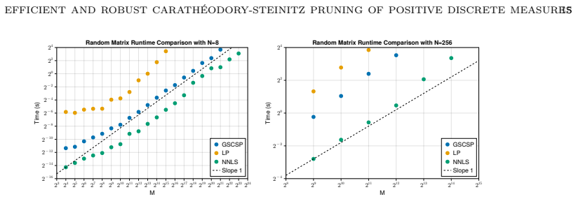
In many applications, one seeks to approximate integration against a positive measure of interest by a positive discrete measure: a numerical quadrature rule with positive weights. One common desired discretization property is moment preservation over a finite dimensional function space, e.g., bounded-degree polynomials. Carath\'{e}odory's theorem asserts that if there is any finitely supported quadrature rule with more nodes than the dimension of the given function space, one can form a smaller (and hence more efficient) positive, nested, quadrature rule that preserves the moments of the original rule. We describe an efficient streaming procedure for Carath\'{e}odory-Steinitz pruning, a numerical procedure that implements Carath\'{e}odory's theorem for this measure compression. The new algorithm makes use of Givens rotations and on-demand storage of arrays to successfully prune very large rules whose storage complexity only depends on the dimension of the function space. This approach improves on a naive implementation of Carath\'{e}odory-Steinitz pruning whose runtime and storage complexity are quadratic and linear, respectively, in the size of the original measure. We additionally prove mathematical stability properties of our method with respect to a set of admissible, total-variation perturbations of the original measure. Our method is compared to two alternative approaches with larger storage requirements: non-negative least squares and linear programming, and we demonstrate comparable runtimes, with improved stability and storage robustness. Finally, we demonstrate practical usage of this algorithm to generate quadrature for discontinuous Galerkin finite element simulations on cut-cell meshes.
Figures


Figures from the paper (6 more)


Reference graph
Works this paper leans on
-
[1]
The proof of Tchakaloff’s Theorem
C. Bayer and J. Teichmann. “The proof of Tchakaloff’s Theorem”. en. In: Proceedings of the American Mathematical Society 134.10 (2006), pp. 3035–
2006
-
[2]
Non-intrusive uncertainty quantification using reduced cubature rules
L. M. M. van den Bos, B. Koren, and R. P. Dwight. “Non-intrusive uncertainty quantification using reduced cubature rules”. In: Journal of Computational Physics 332 (2017), pp. 418–445. issn: 0021-9991. doi: 10 . 1016 / j . jcp . 2016.12.011
2017
-
[3]
Generating Nested Quadrature Rules with Positive Weights based on Arbitrary Sam- ple Sets
L. van den Bos, B. Sanderse, W. Bierbooms, and G. van Bussel. “Generating Nested Quadrature Rules with Positive Weights based on Arbitrary Sam- ple Sets”. In: SIAM/ASA Journal on Uncertainty Quantification 8.1 (2020), pp. 139–169. doi: 10.1137/18M1213373
-
[4]
A fast non-negativity-constrained least squares algo- rithm
R. Bro and S. De Jong. “A fast non-negativity-constrained least squares algo- rithm”. In: Journal of Chemometrics: A Journal of the Chemometrics Society 11.5 (1997), pp. 393–401
1997
-
[5]
Skew-symmetric entropy stable modal discontinuous Galerkin for- mulations
J. Chan. “Skew-symmetric entropy stable modal discontinuous Galerkin for- mulations”. In: Journal of Scientific Computing 81.1 (2019), pp. 459–485
2019
-
[6]
A duality proof of Tchakaloff’s theorem
R. E. Curto and L. A. Fialkow. “A duality proof of Tchakaloff’s theorem”. In: Journal of Mathematical Analysis and Applications 269.2 (2002), pp. 519–
2002
-
[7]
A construction of nonnegative approximate quadratures
P. J. Davis. “A construction of nonnegative approximate quadratures”. In: Mathematics of Computation 21.100 (1967), pp. 578–582. issn: 0025-5718, 1088-6842. doi: 10.1090/S0025-5718-1967-0222534-4
-
[8]
Carath´ eodory bounds for integer cones
F. Eisenbrand and G. Shmonin. “Carath´ eodory bounds for integer cones”. In: Operations Research Letters 34.5 (2006), pp. 564–568. issn: 0167-6377. doi: https://doi.org/10.1016/j.orl.2005.09.008
Show all 31 references
-
[9]
The BR1 scheme is stable for the compressible Navier–Stokes equations
G. J. Gassner, A. R. Winters, F. J. Hindenlang, and D. A. Kopriva. “The BR1 scheme is stable for the compressible Navier–Stokes equations”. In: Journal of Scientific Computing 77.1 (2018), pp. 154–200
2018
-
[10]
A two-dimensional stabilized discontinuous Galerkin method on curvilinear embedded boundary grids
A. Giuliani. “A two-dimensional stabilized discontinuous Galerkin method on curvilinear embedded boundary grids”. In: SIAM Journal on Scientific Computing 44.1 (2022), A389–A415
2022
-
[11]
Constructing Positive Interpolatory Cubature Formulas
J. Glaubitz. “Constructing Positive Interpolatory Cubature Formulas”. In: arXiv:2009.11981 [cs, math] (2020). arXiv: 2009.11981
2009 arXiv
-
[12]
Stable High Order Quadrature Rules for Scattered Data and General Weight Functions
J. Glaubitz. “Stable High Order Quadrature Rules for Scattered Data and General Weight Functions”. In: SIAM Journal on Numerical Analysis 58.4 (2020), pp. 2144–2164. issn: 0036-1429. doi: 10.1137/19M1257901
2020 doi
-
[13]
Construction and application of provable positive and exact cubature formulas
J. Glaubitz. “Construction and application of provable positive and exact cubature formulas”. In: IMA Journal of Numerical Analysis 43.3 (2023), pp. 1616–1652. issn: 0272-4979. doi: 10.1093/imanum/drac017
2023 doi
-
[14]
G. H. Golub and C. F. V. Loan. Matrix Computations (Johns Hopkins Studies in Mathematical Sciences) . 3rd. The Johns Hopkins University Press, 1996. isbn: 0-8018-5414-8
1996
-
[15]
J. S. Hesthaven and T. Warburton. Nodal discontinuous Galerkin methods: algorithms, analysis, and applications . Springer
-
[16]
Karniadakis and S
G. Karniadakis and S. Sherwin. Spectral/hp element methods for computa- tional fluid dynamics . Oxford University Press, USA, 2013. 22 REFERENCES
2013
-
[17]
C. L. Lawson and R. J. Hanson. Solving Least Squares Problems . Society for Industrial and Applied Mathematics, 1995. doi: 10.1137/1.9781611971217. eprint: https://epubs.siam.org/doi/pdf/10.1137/1.9781611971217
1995 doi
-
[18]
JuMP 1.0: Recent improvements to a modeling language for mathemati- cal optimization
M. Lubin, O. Dowson, J. Dias Garcia, J. Huchette, B. Legat, and J. P. Vielma. “JuMP 1.0: Recent improvements to a modeling language for mathemati- cal optimization”. In: Mathematical Programming Computation 15 (2023), pp. 581–589. doi: 10.1007/s12532-023-00239-3
2023 doi
-
[19]
Caratheodory- Tchakaloff Subsampling
F. Piazzon, A. Sommariva, M. Vianello, and M. Vianello. “Caratheodory- Tchakaloff Subsampling”. In: Dolomites Research Notes on Approximation 10.1 (2017). arxiv 1611.02065 [math.NA], pp. 5–14. issn: 20356803. doi: 10. 14658/pupj-drna-2017-1-2
2017 arXiv
-
[20]
A note on Tchakaloff’s Theorem
M. Putinar. “A note on Tchakaloff’s Theorem”. In: Proceedings of the Ameri- can Mathematical Society 125.8 (1997), pp. 2409–2414. issn: 0002-9939, 1088-
1997
-
[21]
Entropy stable reduced order modeling of nonlinear conservation laws using discontinuous Galerkin methods
R. Qu, A. Narayan, and J. Chan. “Entropy stable reduced order modeling of nonlinear conservation laws using discontinuous Galerkin methods”. In:arXiv preprint arXiv:2502.09381 (2025)
2025
-
[22]
Bedingt konvergente Reihen und konvexe Systeme
E. Steinitz. “Bedingt konvergente Reihen und konvexe Systeme.” de. In: Jour- nal f¨ ur die reine und angewandte Mathematik 1913.143 (1913), pp. 128–176. issn: 1435-5345. doi: 10.1515/crll.1913.143.128
1913 doi
-
[23]
An Entropy Stable High-Order Discontinuous Galerkin Method on Cut Meshes
C. G. Taylor and J. Chan. “An Entropy Stable High-Order Discontinuous Galerkin Method on Cut Meshes”. In:arXiv preprint arXiv:2412.13002 (2024)
2024 arXiv
-
[24]
An energy stable high-order cut cell discontinuous Galerkin method with state redistribution for wave propa- gation
C. G. Taylor, L. C. Wilcox, and J. Chan. “An energy stable high-order cut cell discontinuous Galerkin method with state redistribution for wave propa- gation”. In: Journal of Computational Physics 521 (2025), p. 113528
2025
-
[25]
Formules de cubatures m´ ecaniques ` a coefficients non n´ egatifs
V. Tchakaloff. “Formules de cubatures m´ ecaniques ` a coefficients non n´ egatifs”. In: Bull. Sci. Math 81.2 (1957), pp. 123–134
1957
-
[26]
Caratheodory cubature measures
M. Tchernychova. “Caratheodory cubature measures”. http://purl.org/dc/dcmitype/Text. University of Oxford, 2016
2016
-
[27]
A general algorithm for nonnegative quadrature formulas
M. W. Wilson. “A general algorithm for nonnegative quadrature formulas”. In: Mathematics of Computation 23.106 (1969), pp. 253–258. issn: 0025-5718, 1088-6842. doi: 10.1090/S0025-5718-1969-0242374-1
1969 doi
-
[28]
An LP empirical quadrature procedure for re- duced basis treatment of parametrized nonlinear PDEs
M. Yano and A. T. Patera. “An LP empirical quadrature procedure for re- duced basis treatment of parametrized nonlinear PDEs”. In: Computer Meth- ods in Applied Mechanics and Engineering 344 (2019), pp. 1104–1123. issn: 0045-7825. doi: https://doi.org/10.1016/j.cma.2018.02.028...
2019 doi
- [532]
-
[3040]
doi: 10.1090/S0002-9939-06-08249-9
issn: 0002-9939, 1088-6826. doi: 10.1090/S0002-9939-06-08249-9
-
[6826]
doi: 10.1090/S0002-9939-97-03862-8
Reviewed August 4, 2026 · model on record in the stance chip above.
Discussion (0). Continue with ORCID to comment.