REVIEW 3 major objections 5 minor 58 references
Portable 90 mT MRI can image tendons, ligaments, cartilage, and bone in vivo within 15 minutes, and measure their T1 relaxation times.
Reviewed by Pith at T0; open to challenge. T0 means a machine referee read the full paper against a public rubric. the ladder, T0–T4 →
T0 review · deepseek-v4-flash
2026-08-03 21:19 UTC pith:PG42NPVW
load-bearing objection Solid proof-of-concept for ZTE on a Halbach portable scanner; the in-vivo hard-tissue T1 values are preliminary until the phantom-to-in-vivo field-map transfer is validated. the 3 major comments →
Qualitative and quantitative hard-tissue MRI with portable Halbach scanners
The pith
A machine-rendered reading of the paper's core claim, the machinery that carries it, and where it could break.
Core claim
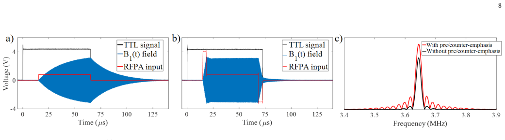
The central discovery is that ZTE-like PETRA imaging can be transplanted from clinical high-field platforms to a portable 90 mT Halbach scanner, provided the sequence is adapted to the hardware's long coil ring-down and strong field inhomogeneity. The authors show that a three-part RF pulse (pre-emphasis, main pulse, counter-emphasis) cuts the electronics dead time, and that an extension of a single-point double-shot protocol yields simultaneous B0 and B1 maps of the imaging volume. Feeding these maps into a model-based algebraic reconstruction removes the geometric distortions and banding artifacts that otherwise plague ZTE data in inhomogeneous fields. With this toolkit, the authors obtain
What carries the argument
PETRA (Pointwise Encoding Time Reduction with Radial Acquisition), a ZTE variant that samples the center of k-space pointwise with short RF pulses and the periphery radially; the paper's contribution is a chain of calibrations around it: RF pulse pre/counter-emphasis to suppress ring-down, an extended SPDS (single-point double-shot) SPRITE protocol to map B0 and B1 fields, and a model-based Kaczmarz (ART) reconstruction whose encoding matrix incorporates those field maps. The same PETRA pair with two flip angles (VFA-PETRA) serves as the T1 relaxometry engine, using the steady-state signal ratio and known field maps to solve for T1 voxelwise.
Load-bearing premise
The load-bearing assumption is that the B0 and B1 field maps measured on a homogeneous phantom after the volunteer's knee is removed, using the same shim settings, faithfully represent the field distributions inside the actual knee — no in-vivo validation of this transfer is presented.
What would settle it
Acquire the same PETRA and VFA-PETRA knee data twice: once reconstructed with the phantom-transferred maps, and once with SPDS field maps acquired while the knee is still in place (e.g., using the knee's own signal or a co-registered phantom). If T1 estimates and image artifacts differ substantially, or if the in-situ maps show gradients in regions where the phantom maps are smooth, the central claim is weakened.
If this is right
- If the approach is correct, portable Halbach scanners could offer a non-ionizing, low-cost alternative to X-rays for evaluating ligaments, tendons, and bone.
- The in-vivo T1 values reported for short-T2 tissues at 90 mT provide a reference that could anchor future low-field relaxometry work and MR fingerprinting at sub-0.1 T.
- The model-based reconstruction framework is transferable: any sequence whose encoding is distorted by measured field maps can be rebuilt in the same way.
- The under-15-minute scan time brings hard-tissue MRI within reach of point-of-care workflows, sports medicine, and home-based monitoring.
Where Pith is reading between the lines
- Our inference: because the field maps used for the in-vivo reconstructions were measured on a phantom after the knee was removed, the results inherit the untested assumption that the knee's presence does not change the field distributions; a direct test with in-situ maps would settle this.
- Our inference: the VFA-PETRA T1 retrieval could be extended to T2* or multi-echo ZTE variants, which the authors mention as future work; a natural next test is to see whether the same framework recovers known T1 values of phantoms under edge-of-bore conditions.
- Our inference: the contrast-enhancement subtractions shown in the paper (flip-angle pairs that highlight ligament, fat, muscle, or cartilage) suggest a vendor-independent 'synthetic contrast' recipe that could be packaged without any quantitative fitting.
Editorial analysis
A structured set of objections, weighed in public.
Referee Report
Summary. This manuscript reports a complete pipeline for zero-echo-time (ZTE) imaging on a portable 90 mT Halbach scanner. The authors implement a PETRA sequence with RF pre/counter-emphasis to shorten the effective dead time, extend a single-point double-shot (SPDS) protocol to obtain B0/B1 maps from a homogeneous phantom, and use model-based ART reconstruction that incorporates these maps into the encoding matrix. A variable-flip-angle (VFA) version of PETRA is then used for T1 mapping. The results show in-vivo knee/ankle images with visible ligaments, tendons, cartilage, and cortical bone, and report T1 values for several soft and hard tissues. The paper claims the first demonstration of ZTE imaging on a Halbach-based portable MRI system and the first in-vivo hard-tissue T1 estimates at B0 < 0.1 T.
Significance. If the quantitative claims are supported, this would be an important advance for portable MRI: it substantially widens the range of pulse sequences and tissue types accessible to low-cost Halbach scanners. The technical contributions — pre/counter-emphasis calibration, SPDS-based simultaneous field mapping, model-based reconstruction, and open-source MaRCoS sequence code — are concrete and reusable. The phantom validation of VFA-PETRA and the benchmark of muscle/fat T1 against RARE/STIR are strong points. However, the headline hard-tissue T1 values depend on an unverified transfer of phantom-acquired B0/B1 maps to in-vivo loading conditions; this needs to be addressed before the quantitative claims can be considered established.
major comments (3)
- [III-F; Eq. (8); Eq. (13)] The in-vivo PETRA and VFA-PETRA reconstructions are corrected with B0/B1 maps acquired from a homogeneous CuSO4 phantom that fully occupies the coil, after removing the knee and re-adjusting impedance matching (Sec. III-F). This transfer is assumed without validation. The knee is smaller, lossy, and contains susceptibility discontinuities near bone/tendon/cartilage; these change both B0 and B1 relative to the phantom, and the change is not controlled by keeping the same shim currents. Because Eqs. (12)-(13) insert these maps into the encoding matrix and Eq. (8) inserts them into the T1 model, any mismatch directly biases both the reconstructed images and the T1 values. The phantom validation in Fig. 7 is self-consistent and does not test the in-vivo loading condition. The agreement for muscle/fat T1 with RARE/STIR is encouraging for large soft-tissue ROIs but cannot validate small short-
- [V-E; Fig. 12] The hard-tissue T1 values are presented as quantitative results, but no reference standard exists for ligament, tendon, cartilage, or cortical bone at this field, and the only quantitative agreement is for muscle/fat. The ROIs are small, and the Discussion itself notes that the meniscus could not be quantified because of insufficient segmentation accuracy. The Gaussian-fit standard deviations in Fig. 12d reflect spatial heterogeneity and noise, not systematic error from B0/B1 transfer, partial volume, or segmenter choice. To support the 'first in-vivo T1' claim, the paper should report repeatability (e.g., repeated scans), segmenter variability, or an explicit error budget. The hard-tissue values should be labeled as provisional estimates until such an analysis is supplied.
- [III-D; III-G] The B0/B1 maps are acquired at 10 mm isotropic resolution and zero-padded/interpolated to the 1.6-2 mm reconstruction grid. This smoothing is likely to miss the local field variations caused by susceptibility interfaces in the knee, which are strongest around exactly the short-T2 tissues the quantitative method targets. The interpolation step in Sec. III-G therefore compounds the phantom-transfer problem. A finer field-map acquisition (or an empirical correction) should be considered, or the resolution-dependence of the T1 estimates should be reported.
minor comments (5)
- [Eq. (1)] The scaling relation is dimensionally opaque; please define the units of T_dead, T_acq, N_max, and FoV_max and state whether the formula is exact or heuristic. As written, the third term inside the parentheses appears to have mixed dimensions.
- [Fig. 7] The text in Sec. IV-D refers to panel (c) as the uncorrected and (e) as the corrected T1 map, while the caption assigns (c) and (d) to maps; renumber the caption/text to match.
- [Disclosures] The disclosure that tissue identification was performed without input from certified radiologists is helpful; it would be better placed in Methods or in the figure captions so that readers of Figs. 8 and 9 are not misled. A review by a radiologist would be even stronger.
- [Introduction / References] The claim of 'first proof of ZTE-like PETRA imaging in a Halbach-based MRI system' should be checked against Ref. [28], which already used short-T2 imaging in a low-field permanent-magnet dental scanner. If Ref. [28] is not Halbach-based, the distinction should be stated explicitly.
- [Various] Minor typographical issues: 'componentes' in the Fig. 1 caption and 'within vivodata' in Sec. II-G should be corrected.
Circularity Check
No significant circularity: field maps are independent phantom calibrations and VFA-PETRA T1 estimates are benchmarked against standard methods.
full rationale
The derivation chain is self-contained. The B0 and B1 maps are obtained from an independent SPDS acquisition on a homogeneous CuSO4 phantom whose T1 was measured independently by inversion recovery (T1 = 12.5 ms). These maps enter the VFA-PETRA model (Eq. 8) as known inputs, with T1 as the only unknown; the phantom-based validation of VFA-PETRA uses the same phantom but is a consistency check, not a construction of the result. The model-based reconstruction (Eqs. 11-13) incorporates the same field maps but does not fit or predefine T1, so no fitted parameter is renamed as a prediction. The VFA-PETRA muscle and fat T1 values are cross-checked against standard RARE/STIR maps, providing an external benchmark. The self-citation to Ref. [30] supplies the SPDS protocol, but the paper re-derives the extension in Sec. II-F and validates it in Figs. 5 and 7, so the central feasibility claim does not reduce to that citation. The phantom-to-in-vivo transfer of field maps is an untested assumption that could bias quantitative T1 values, but that is an external-validity or accuracy risk, not circularity by construction. No equation in the paper reduces a claimed prediction to its own input.
Axiom & Free-Parameter Ledger
free parameters (5)
- Pre/counter-emphasis RF amplitudes and durations =
V_RF0/V_RF1/V_RF2 = 1/0.25/1 a.u., t_RF0/t_RF1/t_RF2 = 4/50/3 µs (imaging) or 3/25/3 µs (shimming)
- Dead time Tdead =
175 µs (knee) to 300 µs (ankle)
- Active shimming currents =
Unspecified (linewidth reduced to 88 ppm)
- B1 scaling map η(r) =
Voxelwise values estimated via Nelder-Mead minimization of Eq. (5)
- Nominal flip angles α_i,nom =
e.g., 10° and 40° for VFA-PETRA
axioms (4)
- domain assumption PETRA gradients act as effective spoilers, establishing an incoherent steady state across all tissues (Eq. 7).
- ad hoc to paper B0 and B1 field maps measured with a homogeneous CuSO4 phantom are representative of the in-vivo knee/ankle configuration when the same shimming settings are used.
- domain assumption The signal observed in PETRA images of the knee/ankle corresponds to the labeled short-T2 tissues (ligaments, tendons, cartilage, bone).
- standard math Standard FFT, Kaczmarz/ART, and steady-state Bloch equations provide valid image reconstruction and T1 fitting tools.
read the original abstract
Purpose: To demonstrate the feasibility of performing in-vivo imaging and quantitative relaxation mapping of soft and hard tissues using a low-cost, portable MRI scanner, and to establish the methodological foundations for zero echo time (ZTE) imaging in systems affected by strong field inhomogeneities. Methods: A complete framework for artifact-free ZTE imaging at low field was developed, including: (i) RF pulse pre/counteremphasis calibration to minimize ring-down and electronics switching time; (ii) an extension of a recent single-point double-shot (SPDS) protocol for simultaneous B0 and B1 mapping; and (iii) a model-based reconstruction incorporating these field maps into the encoding matrix. ZTE imaging and variable flip angle (VFA) T1 mapping were performed on phantoms and in-vivo human knees and ankles, and benchmarked against standard RARE and STIR acquisitions. Results: The optimized PETRA sequence produced 3D images of knees and ankles within clinically compatible times (< 15 min), revealing hard tissues such as ligaments, tendons, cartilage, and bone that are invisible in spin-echo sequences. The extended SPDS method enabled accurate field mapping, while the VFA approach provided the first in-vivo T1 measurements of hard tissues at B0 < 0.1 T. Conclusions: The proposed framework broadens the range of pulse sequences feasible in portable low-field MRI and demonstrates the potential of ZTE for quantitative and structural imaging of musculoskeletal tissues in affordable Halbach-based systems.
Figures



Reference graph
Works this paper leans on
-
[1]
Low-Cost High-Performance MRI,
M. Sarracanie, C. D. LaPierre, N. Salameh, D. E. J. Waddington, T. Witzel, and M. S. Rosen, “Low-Cost High-Performance MRI,” Scientific Reports, vol. 5, no. 1, p. 15177, dec 2015. [Online]. Available: http://www.nature.com/articles/srep15177
2015
-
[2]
Accessible magnetic resonance imaging: A review,
S. Geethanath and J. T. Vaughan, “Accessible magnetic resonance imaging: A review,”Journal of Magnetic Resonance Imaging, vol. 49, 01 2019
2019
-
[3]
On-site construction of a point-of-care low-field MRI system in Africa,
J. Obungoloch, I. Muhumuza, W. Teeuwisse, J. Harper, I. Etoku, R. Asiimwe, P. Tusiime, G. Gombya, C. Mugume, M. H. Namutebi, M. A. Nassejje, M. Nayebare, J. M. Kavuma, B. Bukyana, F. Natukunda, P. Ninsiima, A. Muwanguzi, P. Omadi, M. van Gijzen, S. J. Schiff, A. Webb, and T. O’Reilly, “On-site construction of a point-of-care low-field MRI system in Africa...
2023
-
[4]
L. L. Wald, P. C. McDaniel, T. Witzel, J. P. Stockmann, and C. Z. Cooley, “Low-cost and portable MRI,”Journal of Magnetic Resonance Imaging, vol. 52, no. 3, pp. 686–696, 2020. [Online]. Available: https://onlinelibrary.wiley.com/doi/abs/10.1002/jmri.26942
-
[5]
Portable magnetic resonance imaging of patients indoors, outdoors and at home,
T. Guallart-Naval, J. Algarin, R. Pellicer-Guridi, F. Galve, Y. Vives- Gilabert, R. Bosch, E. Pallas, J. M. Gonzalez, J. Rigla, P. Martinez, F. J. Lloris, J. Borreguero Morata, A. Marcos-Perucho, V. Negnevitsky, L. Marti-Bonmati, A. Rios, J. Benlloch, and J. Alonso, “Portable magnetic resonance imaging of patients indoors, outdoors and at home,”Scientific...
2022
-
[6]
Tackling SNR at low-field: a review of hardware approaches for point-of-care systems,
A. Webb and T. O’Reilly, “Tackling SNR at low-field: a review of hardware approaches for point-of-care systems,”Magnetic Resonance Materials in Physics, Biology and Medicine, vol. 36, 05 2023
2023
-
[7]
Deconstructing and reconstructing MRI hardware,
T. O’Reilly and A. Webb, “Deconstructing and reconstructing MRI hardware,”Journal of Magnetic Resonance, vol. 306, pp. 134–138,
-
[8]
MRI at low field: A review of software solutions for improving SNR,
R. Ayde, M. Vornehm, Y. Zhao, F. Knoll, E. X. Wu, and M. Sarracanie, “MRI at low field: A review of software solutions for improving SNR,”NMR in Biomedicine, vol. 38, no. 1, p. e5268, 2025. [Online]. Available: https://analyticalsciencejournals.onlinelibrary.wiley.com/doi/ abs/10.1002/nbm.5268
doi:10.1002/nbm.5268 2025
-
[9]
Design of permanent multipole magnets with oriented rare earth cobalt material,
K. Halbach, “Design of permanent multipole magnets with oriented rare earth cobalt material,”Nuclear Instruments and Methods, vol. 169, no. 1, pp. 1–10, 1980
1980
-
[10]
In vivo 3D brain and extremity MRI at 50 mT using a permanent magnet Halbach array,
T. O’Reilly, W. M. Teeuwisse, D. Gans, K. Koolstra, and A. G. Webb, “In vivo 3D brain and extremity MRI at 50 mT using a permanent magnet Halbach array,”Magnetic Resonance in Medicine, p. mrm.28396, jul 2020
2020
-
[11]
A portable scanner for magnetic resonance imaging of the brain,
C. Z. Cooley, P. C. McDaniel, J. P. Stockmann, S. A. Srinivas, S. F. Cauley, M. ´Sliwiak, C. R. Sappo, C. F. Vaughn, B. Guerin, M. S. Rosen, M. H. Lev, and L. L. Wald, “A portable scanner for magnetic resonance imaging of the brain,”Nature Biomedical Engineering 2020 5:3, vol. 5, no. 3, pp. 229–239, nov 2020
2020
-
[12]
Elliptical Halbach magnet and gradient modules for low-field portable magnetic resonance imaging,
F. Galve, E. Pall ´as, T. Guallart-Naval, P. Garc ´ıa-Crist´obal, P. Mart´ınez, J. M. Algar ´ın, J. Borreguero, R. Bosch, F. Juan-Lloris, J. M. Benlloch, and J. Alonso, “Elliptical Halbach magnet and gradient modules for low-field portable magnetic resonance imaging,”NMR in Biomedicine, p. e5258, 2024. [Online]. Available: https://analyticalsciencejournal...
doi:10.1002/nbm.5258 2024
-
[13]
Development of a small car-mounted magnetic resonance imaging system for human elbows using a 0.2 T permanent magnet,
M. Nakagomi, M. Kajiwara, J. Matsuzaki, K. Tanabe, S. Hoshiai, Y. Okamoto, and Y. Terada, “Development of a small car-mounted magnetic resonance imaging system for human elbows using a 0.2 T permanent magnet,”Journal of Magnetic Resonance, vol. 304, pp. 1–6, jul 2019
2019
-
[14]
De- velopment of a Car-mounted Mobile MR Imaging System for Diagnosis of Sports-related Wrist Injury,
T. Miyasaka, M. Kajiwara, A. Kawasaki, Y. Okamoto, and Y. Terada, “De- velopment of a Car-mounted Mobile MR Imaging System for Diagnosis of Sports-related Wrist Injury,”Magnetic Resonance in Medical Sciences, vol. 22, 04 2022
2022
-
[15]
Portable MRI for Major Sporting Events – a Case Study on the MotoGP World Championship,
J. M. Algar ´ın, T. Guallart-Naval, E. G. Orqu´ın, R. Bosch, F. Juan-Lloris, E. Pall ´as, J. P. Rigla, P. Mart ´ınez, J. Borreguero, R. Alamar, L. Mart ´ı- Bonmat´ı, J. M. Benlloch, F. Galve, and J. Alonso, “Portable MRI for Major Sporting Events – a Case Study on the MotoGP World Championship,” Portable MRI Journal, February 2024. [Online]. Available: ht...
2024
-
[16]
E. L. Hahn, “Spin Echoes,”Phys. Rev., vol. 80, pp. 580–594, Nov 1950. [Online]. Available: https://link.aps.org/doi/10.1103/PhysRev.80.580
-
[17]
Effects of diffusion on free precession in nuclear magnetic resonance experiments,
H. Y. Carr and E. M. Purcell, “Effects of diffusion on free precession in nuclear magnetic resonance experiments,”Physical Review, vol. 94, no. 3, pp. 630–638, 1954
1954
-
[18]
Magnetic Resonance Imaging of Hard Tissues and Hard Tissue Engineered Bio-substitutes,
S. Mastrogiacomo, W. Dou, J. A. Jansen, and X. F. Walboomers, “Magnetic Resonance Imaging of Hard Tissues and Hard Tissue Engineered Bio-substitutes,”Molecular Imaging and Biology, vol. 21, no. 6, pp. 1003–1019, dec 2019. [Online]. Available: http: //link.springer.com/10.1007/s11307-019-01345-2
-
[19]
Quantitative mri for evaluation of musculoskeletal disease: Cartilage and muscle composition, joint inflammation, and biomechanics in osteoarthritis,
B. Eck, M. Yang, J. Elias, C. Winalski, F. Altahawi, N. Subhas, and X. Li, “Quantitative mri for evaluation of musculoskeletal disease: Cartilage and muscle composition, joint inflammation, and biomechanics in osteoarthritis,”Investigative Radiology, vol. Publish Ahead of Print, 09 2022
2022
-
[20]
Magnetic Resonance: An Introduction to Ultrashort TE (UTE) Imaging,
M. D. Robson, P. D. Gatehouse, M. Bydder, and G. M. Bydder, “Magnetic Resonance: An Introduction to Ultrashort TE (UTE) Imaging,”Journal of Computer Assisted Tomography, vol. 27, no. 6, pp. 825–846, November 2003
2003
-
[21]
Ultra-fast imaging using low flip angles and fids,
D. P. Madio and I. J. Lowe, “Ultra-fast imaging using low flip angles and fids,”Magnetic Resonance in Medicine, vol. 34, no. 4, pp. 525–529, 1995. [Online]. Available: https://onlinelibrary.wiley.com/doi/ abs/10.1002/mrm.1910340407
-
[22]
Fast and quiet MRI using a swept radiofrequency,
D. Idiyatullin, C. Corum, J.-Y. Park, and M. Garwood, “Fast and quiet MRI using a swept radiofrequency,”Journal of Magnetic Resonance, vol. 181, no. 2, pp. 342–349, 2006. [Online]. Available: https://www.sciencedirect.com/science/article/pii/S1090780706001479
2006
-
[23]
A clinically-recommended MR whole 15 lung imaging protocol using free-breathing 3D isotropic zero echo time sequence,
Q. Lin, C. Cheng, Y. Bao, W. V. Liu, L. Zhang, Z. Cai, Q. Wan, C. Sun, X. Li, and Y. Deng, “A clinically-recommended MR whole 15 lung imaging protocol using free-breathing 3D isotropic zero echo time sequence,”Heliyon, vol. 10, no. 13, p. e34098, 2024. [Online]. Available: https://www.sciencedirect.com/science/article/pii/S2405844024101296
2024
-
[24]
Articular cartilage assessment using ultrashort echo time mri: A review,
A. M. Afsahi, S. Sedaghat, D. Moazamian, G. Afsahi, J. S. Athertya, H. Jang, and Y.-J. Ma, “Articular cartilage assessment using ultrashort echo time mri: A review,”Frontiers in Endocrinology, vol. Volume 13 - 2022, 2022. [Online]. Available: https://www.frontiersin.org/journals/ endocrinology/articles/10.3389/fendo.2022.892961
arXiv 2022
-
[25]
Tendon evaluation with ultrashort echo time (ute) mri: a systematic review,
B. S. Malhi, H. Jang, M. S. Malhi, D. B. Berry, and S. Jerban, “Tendon evaluation with ultrashort echo time (ute) mri: a systematic review,”Frontiers in Musculoskeletal Disorders, vol. Volume 2 - 2024, 2024. [Online]. Available: https://www.frontiersin.org/journals/ musculoskeletal-disorders/articles/10.3389/fmscd.2024.1324050
arXiv 2024
-
[26]
High-resolution ZTE imaging of human teeth,
M. Weiger, K. P. Pruessmann, A.-K. Bracher, S. K ¨ohler, V. Lehmann, U. Wolfram, F. Hennel, and V. Rasche, “High-resolution ZTE imaging of human teeth,”NMR in Biomedicine, vol. 25, no. 10, pp. 1144–1151, oct
-
[27]
Dental magnetic resonance imaging: making the invisible visible,
D. Idiyatullin, C. Corum, S. Moeller, H. S. Prasad, M. Garwood, and D. R. Nixdorf, “Dental magnetic resonance imaging: making the invisible visible,”Journal of endodontics, vol. 37, no. 6, pp. 745–752, 2011
2011
-
[28]
Simultaneous imaging of hard and soft biological tissues in a low-field dental MRI scanner,
J. M. Algar ´ın, E. D´ıaz-Caballero, J. Borreguero, F. Galve, D. Grau-Ruiz, J. P. Rigla, R. Bosch, J. M. Gonz´alez, E. Pall´as, M. Corber´an, C. Gramage, S. Aja-Fern´andez, A. R´ıos, J. M. Benlloch, and J. Alonso, “Simultaneous imaging of hard and soft biological tissues in a low-field dental MRI scanner,”Scientific Reports, vol. 10, no. 1, p. 21470, 2020...
-
[29]
Ultrashort echo time imaging using pointwise encoding time reduction with radial acquisition (PETRA),
D. M. Grodzki, P. M. Jakob, and B. Heismann, “Ultrashort echo time imaging using pointwise encoding time reduction with radial acquisition (PETRA),”Magnetic Resonance in Medicine, vol. 67, no. 2, pp. 510–518, feb 2012
2012
-
[30]
Zero-echo-time sequences in highly inhomogeneous fields,
J. Borreguero, F. Galve, J. M. Algar ´ın, and J. Alonso, “Zero-echo-time sequences in highly inhomogeneous fields,”Magnetic Resonance in Medicine, vol. 93, no. 3, pp. 1190–1204, 2025. [Online]. Available: https://onlinelibrary.wiley.com/doi/abs/10.1002/mrm.30352
-
[31]
MRI with zero echo time: Hard versus sweep pulse excitation,
M. Weiger, K. P. Pruessmann, and F. Hennel, “MRI with zero echo time: Hard versus sweep pulse excitation,”Magnetic Resonance in Medicine, vol. 66, no. 2, pp. 379–389, aug 2011. [Online]. Available: http://doi.wiley.com/10.1002/mrm.22799
-
[32]
P. A. Bottomley, T. H. Foster, R. E. Argersinger, and L. M. Pfeifer, “A review of normal tissue hydrogen NMR relaxation times and relaxation mechanisms from 1–100 MHz: Dependence on tissue type, NMR frequency, temperature, species, excision, and age,”Medical Physics, vol. 11, no. 4, pp. 425–448, 1984. [Online]. Available: https://aapm.onlinelibrary.wiley....
-
[33]
Magnetic field dependence of proton spin-lattice relaxation times,
J.-P. Korb and R. G. Bryant, “Magnetic field dependence of proton spin-lattice relaxation times,”Magnetic Resonance in Medicine, vol. 48, no. 1, pp. 21–26, 2002. [Online]. Available: https: //onlinelibrary.wiley.com/doi/abs/10.1002/mrm.10185
-
[34]
Magnetic field and tissue dependencies of human brain longitudinal 1H2O relaxation in vivo,
W. D. Rooney, G. Johnson, X. Li, E. R. Cohen, S.-G. Kim, K. Ugurbil, and C. S. Springer Jr., “Magnetic field and tissue dependencies of human brain longitudinal 1H2O relaxation in vivo,”Magnetic Resonance in Medicine, vol. 57, no. 2, pp. 308–318, 2007. [Online]. Available: https://onlinelibrary.wiley.com/doi/abs/10.1002/mrm.21122
-
[35]
In vivo𝑇 1 and𝑇 2 relaxation time maps of brain tissue, skeletal muscle, and lipid measured in healthy volunteers at 50 mT,
T. O’Reilly and A. G. Webb, “In vivo𝑇 1 and𝑇 2 relaxation time maps of brain tissue, skeletal muscle, and lipid measured in healthy volunteers at 50 mT,”Magnetic Resonance in Medicine, vol. 87, no. 2, pp. 884–895, feb 2021
2021
-
[36]
M. Sarracanie, “Fast Quantitative Low-Field Magnetic Resonance Imag- ing With OPTIMUM - Optimized Magnetic Resonance Fingerprinting Using a Stationary Steady-State Cartesian Approach and Accelerated Acquisition Schedules,”Investigative Radiology, 2021
2021
-
[37]
Magnetic resonance fingerprinting,
D. Ma, V. Gulani, N. Seiberlich, K. Liu, J. L. Sunshine, J. L. Duerk, and M. A. Griswold, “Magnetic resonance fingerprinting,”Nature, vol. 495, no. 7440, pp. 187–192, Mar. 2013
2013
-
[38]
Rapid calculation of T1 using variable flip angle gradient refocused imaging,
E. K. Fram, R. J. Herfkens, G. Johnson, G. H. Glover, J. P. Karis, A. Shimakawa, T. G. Perkins, and N. J. Pelc, “Rapid calculation of T1 using variable flip angle gradient refocused imaging,”Magnetic Resonance Imaging, vol. 5, no. 3, pp. 201–208, 1987. [Online]. Available: https://www.sciencedirect.com/science/article/pii/0730725X8790021X
arXiv 1987
-
[39]
R. K. Gupta, “A new look at the method of variable nutation angle for the measurement of spin-lattice relaxation times using fourier transform NMR,”Journal of Magnetic Resonance (1969), vol. 25, no. 1, pp. 231–235, 1977. [Online]. Available: https: //www.sciencedirect.com/science/article/pii/002223647790138X
arXiv 1969
-
[40]
D. F. Alamidi, A. Smailagic, A. W. Bidar, N. S. Parker, M. Olsson, P. D. Hockings, K. M. Lagerstrand, and L. E. Olsson, “Variable flip angle 3D ultrashort echo time (UTE) T1 mapping of mouse lung: A repeatability assessment,”Journal of Magnetic Resonance Imaging, vol. 48, no. 3, pp. 846–852, 2018. [Online]. Available: https://onlinelibrary.wiley.com/doi/a...
-
[41]
Silent T1 mapping using the variable flip angle method with B1 correction,
E. Ljungberg, T. Wood, A. B. Solana, S. Kolind, S. C. R. Williams, F. Wiesinger, and G. J. Barker, “Silent T1 mapping using the variable flip angle method with B1 correction,”Magnetic Resonance in Medicine, vol. 84, no. 2, pp. 813–824, 2020. [Online]. Available: https://onlinelibrary.wiley.com/doi/abs/10.1002/mrm.28178
-
[42]
T1 Mapping using variable flip angle SPGR data with flip angle correction,
G. Liberman, Y. Louzoun, and D. Ben Bashat, “T1 Mapping using variable flip angle SPGR data with flip angle correction,”Journal of Magnetic Resonance Imaging, vol. 40, no. 1, pp. 171–180, 2014. [Online]. Available: https://onlinelibrary.wiley.com/doi/abs/10.1002/jmri.24373
-
[43]
Analysis of the Precision of Variable Flip Angle T1 Mapping with Emphasis on the Noise Propagated from RF Transmit Field Maps,
Y. Lee, M. Callaghan, and Z. Nagy, “Analysis of the Precision of Variable Flip Angle T1 Mapping with Emphasis on the Noise Propagated from RF Transmit Field Maps,”Frontiers in Neuroscience, vol. 11, 03 2017
2017
-
[44]
B1-corrected breast T1 mapping at ultralow field,
S. Shen, N. Koonjoo, S. E. Ogier, T. Boele, M. A. Saksena, K. E. Keenan, and M. S. Rosen, “B1-corrected breast T1 mapping at ultralow field,”Magnetic Resonance in Medicine, vol. 94, no. 5, pp. 1900–1912, 2025. [Online]. Available: https: //onlinelibrary.wiley.com/doi/abs/10.1002/mrm.30602
-
[45]
Characterizing the Human Body as a Monopole Antenna,
B. Kibret, A. K. Teshome, and D. T. H. Lai, “Characterizing the Human Body as a Monopole Antenna,”IEEE Transactions on Antennas and Propagation, vol. 63, no. 10, pp. 4384–4392, 2015
2015
-
[46]
Electromagnetic noise character- ization and suppression in low-field mri systems,
T. Guallart-Naval and J. Alonso, “Electromagnetic noise character- ization and suppression in low-field mri systems,”arXiv preprint arXiv:2507.20413, 2025
arXiv 2025
-
[47]
Benchmarking the performance of a low-cost magnetic resonance control system at multiple sites in the open MaRCoS community,
T. Guallart-Naval, T. O’Reilly, J. M. Algar´ın, R. Pellicer-Guridi, Y. Vives- Gilabert, L. Craven-Brightman, V. Negnevitsky, B. Menk¨ uc, F. Galve, J. P. Stockmann, A. Webb, and J. Alonso, “Benchmarking the performance of a low-cost magnetic resonance control system at multiple sites in the open MaRCoS community,”NMR in Biomedicine, vol. 36, no. 1, p. e4825,
-
[48]
MaRCoS, an open- source electronic control system for low-field MRI,
V. Negnevitsky, Y. Vives-Gilabert, J. M. Algar ´ın, L. Craven- Brightman, R. Pellicer-Guridi, T. O’Reilly, J. P. Stockmann, A. Webb, J. Alonso, and B. Menk¨ uc, “MaRCoS, an open- source electronic control system for low-field MRI,”Journal of Magnetic Resonance, vol. 350, p. 107424, 2023. [Online]. Available: https://www.sciencedirect.com/science/article/p...
2023
-
[49]
MaRGE: A graphical environment for MaRCoS,
J. M. Algar ´ın, T. Guallart-Naval, J. Borreguero, F. Galve, and J. Alonso, “MaRGE: A graphical environment for MaRCoS,”Journal of Magnetic Resonance, vol. 361, p. 107662, 2024. [Online]. Available: https://www.sciencedirect.com/science/article/pii/S1090780724000466
2024
-
[50]
Marcos graphical environment,
“Marcos graphical environment,” 2025, accessed: 2025-03-03. [Online]. Available: https://github.com/mriLab-i3M/MaRGE
2025
-
[51]
Practical method for RF pulse distortion compensation using multiple square pulses for low-field MRI,
Y. Ha, K. Selvaganesan, B. Wu, K. Hancock, C. Rogers, S. Hossein- nezhadian, and G. Galiana, “Practical method for RF pulse distortion compensation using multiple square pulses for low-field MRI,”PLOS ONE, vol. 17, p. e0273432, 09 2022
2022
-
[52]
Single point imaging with radial acquisition and compressed sensing,
S. Ilbey, P. M. Jungmann, J. Fischer, M. Jung, M. Bock, and A. C. ¨Ozen, “Single point imaging with radial acquisition and compressed sensing,”Magnetic Resonance in Medicine, vol. 87, no. 6, pp. 2685–2696, 2022. [Online]. Available: https://onlinelibrary.wiley.com/ doi/abs/10.1002/mrm.29156
-
[53]
Ultrashort echo time (UTE) imaging using gradient pre-equalization and compressed sensing,
H. T. Fabich, M. Benning, A. J. Sederman, and D. J. Holland, “Ultrashort echo time (UTE) imaging using gradient pre-equalization and compressed sensing,”Journal of Magnetic Resonance, vol. 245, pp. 116–124, 2014. [Online]. Available: https://www.sciencedirect.com/ science/article/pii/S1090780714001840
2014
-
[54]
Angen ¨aherte Aufl ¨osung von Systemen linearer Gleichun- gen,
S. Kaczmarz, “Angen ¨aherte Aufl ¨osung von Systemen linearer Gleichun- gen,”Bulletin International de l’Academie Polonaise des Sciences et des Lettres., vol. 35, pp. 355–357, 1937
1937
-
[55]
Nonlocal transform-domain filter for volumetric data denoising and reconstruction,
M. Maggioni, V. Katkovnik, K. Egiazarian, and A. Foi, “Nonlocal transform-domain filter for volumetric data denoising and reconstruction,” IEEE Transactions on Image Processing, vol. 22, no. 1, pp. 119–133, 2013
2013
-
[2012]
Available: http://doi.wiley.com/10.1002/nbm.2783
[Online]. Available: http://doi.wiley.com/10.1002/nbm.2783
-
[2019]
Available: https://www.sciencedirect.com/science/article/ pii/S1090780719301363
[Online]. Available: https://www.sciencedirect.com/science/article/ pii/S1090780719301363
-
[2023]
Available: https://analyticalsciencejournals.onlinelibrary
[Online]. Available: https://analyticalsciencejournals.onlinelibrary. wiley.com/doi/abs/10.1002/nbm.4825
discussion (0)
Sign in with ORCID, Apple, or X to comment. Anyone can read and Pith papers without signing in.