REVIEW 3 major objections 4 minor 71 references
Stochastic Sequential Quadratic Programming for Optimization with Functional Constraints
T0 review · 3 major / 4 minor · reviewed 2026-08-03 · deepseek-v4-flash
Pith's one-line read A stochastic SQP framework solves convex problems with functional constraints without projections or bounded-gradient assumptions, at oracle rates matching unconstrained SGD.
desk verdict Genuinely new stochastic SQP framework; the constraint-violation bound in Theorem 1 is vacuous at the stated parameter setting, but the fix is simple and the paper deserves refereeing. read the letter →
The pith
A machine-rendered reading of the paper's core claim, the machinery that carries it, and where it could break.
The reading
What carries the argument
The central objects are the exact-penalty reformulation and the stochastic prox-linear update. Reformulating (P) as min_x f(x)+h(x)+γ max_k[g_k(x)]_+ turns the functional constraints into a non-smooth composite objective. The prox-linear update linearizes f and each g_k around the current iterate but keeps h and the max operator intact, producing a strongly convex diagonal QP that can be solved without projection. The proof machinery is a one-step inequality (Lemma 2) that couples objective decrease with a Bregman-divergence control of gradient noise, bounding the noise only at the optimum x* rather than globally.
What would settle it
Take a two-variable problem with a single constraint g(x)=x₁²−1 on x₁∈[−2,2] with a known Slater margin, run SSQP with γ set to exactly B̃/ν (the algorithm's stated setting), and check whether the constraint-violation bound (17) holds; the theorem requires γ > B̃/ν, so with equality the right-hand side is infinite and the bound must be adjusted. A sharper test: compute the empirical SFO complexity on a smooth but unbounded-gradient objective (e.g., f(x)=x² with stochastic samples) and check whether it follows the predicted O(1/ε²) in the convex case or O(1/ε) in the strongly convex case; any s
Extended reading notes
Core claim
Under standard smoothness and convexity, the exact-penalty reformulation F(x)=f(x)+h(x)+γ max_k[g_k(x)]_+ is equivalent to the constrained problem (P) once γ ≥ B̃/ν, where ν is the Slater margin and B̃ the objective gap at a Slater point. SSQP applies a stochastic prox-linear step to this F, solving at each iteration a diagonal quadratic program whose constraints are linearizations of the g_k. Theorem 1 gives E[F(x̄_T)]−F(x*) ≤ (2/√T) max{2Lδ0, σ√δ0} and a constraint-violation bound of order 1/√T, with no bounded-gradient assumption. Theorem 2 shows SSQP-Skip needs only O(1/√ε) calls to the quadratic-programming oracle for strongly convex objectives. Theorem 3 gives VARAS an SFO complexity o
Load-bearing premise
The equivalence of the penalty reformulation and the stated rates depend on knowing the Slater margin ν and the optimality gap B̃ at a Slater point in advance, so that γ can be set to at least B̃/ν; if the Slater data is unavailable and γ is chosen by guesswork, the stated constants and feasibility guarantees no longer hold.
Editorial extensions
If this is right
- SSQP attains O(1/ε²) SFO complexity for convex objectives and O(1/ε) for strongly convex objectives, matching known primal–dual and primal methods while avoiding projections and bounded-subgradient assumptions.
- Constraint violation at the averaged iterate is bounded by O(1/√T) whenever γ > B̃/ν, so feasibility is approached at the same rate as optimality.
- SSQP-Skip reduces quadratic-programming oracle calls to O(1/ε^{1/4}) in the strongly convex case while preserving SFO complexity, useful when solving QPs is expensive.
- VARAS matches unconstrained accelerated variance-reduced rates—O(√(nD0)/ε) SFO complexity for convex objectives and O(n log n + √(nκ) log(1/ε)) for strongly convex objectives—for finite-sum problems with functional constraints.
- The analysis framework extends naturally to streaming and real-time settings, where tracking performance can be studied with similar tools.
Reading between the lines
- The diagonal-QP structure suggests that a single-constraint variant, or a variant that samples one constraint per iteration, may inherit similar rates while reducing per-iteration cost from O(m³) to O(m); the paper leaves this as an open problem.
- Because the guarantees hinge on γ ≥ B̃/ν, an adaptive rule that grows γ from the dual values of the per-iteration subproblem—standard in SQP practice—could make the method parameter-free in practice; the paper notes this as future work.
- If the one-step inequality transports to nonconvex functional constraints, a prox-linear analysis could yield stationarity guarantees at similar oracle complexity, though global optimality would be lost.
- The rates suggest that constrained and unconstrained stochastic optimization no longer have a first-order oracle gap when functional constraints are explicit; this could change practical algorithm selection for constrained least-squares and set-membership filtering.
Signed reviews
Editorial analysis
A structured set of objections, weighed in public.
Referee Report
Summary. This paper develops stochastic sequential quadratic programming (SSQP) for convex optimization problems with nonlinear functional constraints. The method uses an exact l_infinity penalty reformulation and a prox-linear / stochastic proximal-gradient update, solving a diagonal QP at each iteration and avoiding projections onto the feasible set. The authors prove O(1/sqrt(T)) objective-gap and constraint-violation bounds for convex objectives, O(1/T) distance bounds for strongly convex objectives, a QP-skipping variant (SSQP-Skip), and an accelerated variance-reduced finite-sum variant (VARAS) with rates matching unconstrained accelerated methods. Numerical experiments on Zermelo trajectory generation and constrained regression compare favorably with APriD, GOCO, and PDSS.
Significance. If correct, this is a substantial contribution: it would be the first projection-free and bounded-gradient-free method achieving these oracle complexities for stochastic convex functional-constrained optimization. The proofs are largely self-contained, with explicit one-step inequalities (Lemmas 1, 2, and 5) and telescoping arguments in Appendices B-D. The VARAS extension is technically nontrivial and correctly leverages the VARAG framework. The numerical comparison against three published baselines on real datasets is a strength. However, the current statement has a mismatch between the theorem and the algorithm for the constraint-violation bound, and the violation metric in Theorem 1 is the max positive constraint value rather than the sum used in the epsilon-optimality definition; these issues need to be fixed before the result can be accepted.
major comments (3)
- [Section III-A, Theorem 1, Eq. (17) and Eq. (64); Algorithm 1] Algorithm 1 sets gamma = B_tilde/nu, but Theorem 1's constraint-violation bound (17) divides by (gamma - B_tilde/nu). At the stated gamma the denominator is zero, and the proof step (64) only yields (gamma - B_tilde/nu) E[w_T] <= ..., which is vacuous at equality. Since constraint violation is half of the epsilon-optimality definition (2), this is load-bearing. The fix is straightforward: either set gamma = (1+delta) B_tilde/nu with delta>0 and restate the theorem, or derive E[w_T] <= (E[F(x_bar_T)]-F(x_star))/gamma from the already-proved objective gap. As written, the theorem and algorithm are inconsistent.
- [Section I, Eq. (2); Section III-A, Theorem 1; Section IV, Theorem 3] The epsilon-optimality criterion (2) is stated with the sum of positive parts, sum_k E[(g_k(x))_+]. However, Theorem 1 bounds only max_k E[(g_k(x_bar_T))_+] (Eq. (17)), and no conversion to the sum is provided. Since sum_k E[(g_k)_+] can be up to m times max_k E[(g_k)_+], the stated SFO complexity does not directly imply the claimed epsilon-optimality criterion unless an extra factor depending on m is introduced. Theorem 3 similarly gives objective-gap and distance bounds but does not state a constraint-violation bound, so the claim that VARAS solves (P) in the sense of (2) is not fully supported. The authors should either change the definition of constraint violation to the max metric or state the additional m-dependent factor in the complexity bounds.
- [Section II-A, Assumption A1; Section II-B] The Slater data (nu, B_tilde) are assumed known in Algorithm 1 and in all complexity bounds, yet the text in Section II-A notes that these 'must be found by parameter tuning.' If only a feasible point with unknown margin is available, the stated gamma cannot be computed, and the constants in the theorem (through L = max{gamma L_g, L_f}) change. This is a limitation of the practical applicability of the stated guarantees. It should be explicitly listed as a limitation or an additional knowledge assumption at the start, rather than left as an aside.
minor comments (4)
- [Theorem 2, display after Eq. (22)] The displayed SFO and QMO complexity formulas are garbled: 'O(σ2/µ2ǫ + κ2 κ√δ0+σ√ǫ)' and the QMO expression need proper parentheses and denominators. They should read, for example, O(σ^2/(µ^2 ε) + κ^2(κ√δ0+σ)/√ε) and correspondingly for the QMO bound.
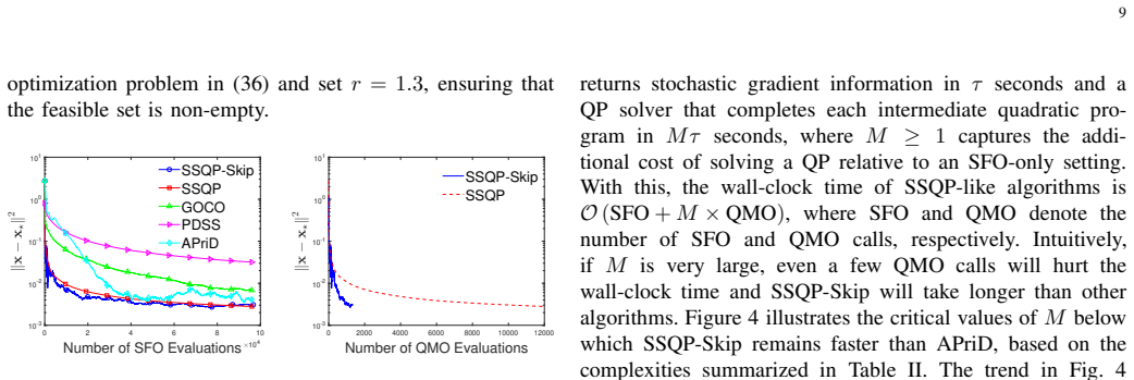
- [Section V-B and Figure 4] The crossover analysis in Figure 4 is described only in words. Since the paper already defines M as the per-QP cost relative to an SFO call, a short formula or table of the critical M values would make the claim more precise and reproducible.
- [Appendix B, proof of Lemma 2] The step size condition in Lemma 2 is stated as η_t ≤ 1/(2(L_f + max{γL_g,L_f})). The proof actually uses the slightly more transparent conditions η_t ≤ 1/(2(L_f+γL_g)) and η_t ≤ 1/(4L_f). Stating all three conditions or adding a one-line derivation would improve readability.
- [Section II-B, paragraph after Eq. (13)] The sentence 'For γ = B̃/ν ≥ ||µ⋆||_1' should clarify that equality is allowed as a limiting case; if γ = ||µ⋆||_1 exactly, the argument still yields v⋆=0 but the accompanying text could be misread as requiring strict inequality.
Circularity Check
No significant circularity: the rate claims are derived from stated assumptions; the Theorem 1 / Algorithm 1 gamma mismatch is a correctness gap, not a circular reduction.
full rationale
The derivation chain is self-contained rather than circular. The central convergence bounds (16)-(18), (22), and (29)-(33) are obtained from one-step inequalities (Lemmas 2, 4, 5) built on smoothness, convexity, the Slater condition, and the noise assumption; none of the inequalities assumes its own conclusion. Theorem 3's appeal to VARAG [35] is external (Lan-Li-Zhou, not the present authors) and is used only for epoch-acceleration bookkeeping after Lemma 5 supplies the required one-step inequality. Self-citations [30], [40], [41], [42], [48] appear only in related-work/comparison contexts and are not load-bearing in the rate proofs. Experimental hyperparameters are tuned separately and compared against published baselines, so no fitted input is renamed as a prediction. The one flagged defect is a correctness gap, not circularity: Algorithm 1 fixes gamma = Btilde/nu, while the constraint-violation bound (17) is stated as E[max_k{[g_k(xbar_T)]_+}] <= 2/((gamma - Btilde/nu) sqrt(T)) max{...}, and the proof's equation (64) indeed requires gamma > Btilde/nu to divide by (gamma - Btilde/nu). The paper itself acknowledges that nu and Btilde 'must be found by parameter tuning' (Sec. II-A). This makes the displayed constant unattained at the stated algorithm setting and is repairable by taking gamma = (1+delta)Btilde/nu or by bounding E[w_T] <= (E[F(xbar_T)] - F(x*))/gamma from the already-proved objective gap. Since this is an algorithmic inconsistency rather than an equivalence between a claimed result and an input, it does not constitute circularity.
Assumptions & free parameters
free parameters (3)
- exact penalty parameter γ =
theory: γ = B̃/ν; experiments: 6×10^5, 10^6, 10^3, 10^5
- SSQP step size η0 =
η0 = min{√δ0/(2σ), 1/(4L)}; experiments: 0.009
- VARAS smoothness/strong-convexity constants (Lγ, μ) =
experiments: Lγ = 350, μ = 0.8 / 0.85
assumptions (6)
- domain assumption A1: Slater condition with known ν and B̃
- domain assumption A2: fi and gk are proper, closed, convex, and L-smooth; f is μ-strongly convex
- domain assumption A3: bounded gradient noise at the optimum, E‖∇f(x*)−∇f_i(x*)‖² ≤ σ²
- standard math Exact penalty equivalence for γ ≥ B̃/ν
- domain assumption SFO oracle returns ∇f_i(x) and all {g_k(x), ∇g_k(x)}; QMO solves each QP subproblem
- standard math External correctness of VARAG and ProxSkip analyses
Cite this review
Pith. "Pith review of Stochastic Sequential Quadratic Programming for Optimization with Functional Constraints." pith.science (2026). https://pith.science/paper/UO46PKZC
@misc{pith2026251120178,
  author       = {Pith},
  title        = {Pith review of: Stochastic Sequential Quadratic Programming for Optimization with Functional Constraints},
  year         = {2026},
  howpublished = {\url{https://pith.science/paper/UO46PKZC}},
  note         = {Machine review of arXiv:2511.20178}
}
read the original abstract
Stochastic convex optimization problems with nonlinear functional constraints are ubiquitous in signal processing applications including constrained least-squares, set-membership adaptive filtering, and trajectory optimization under uncertain fields. The presence of non-linear functional constraints renders the traditional projected stochastic gradient descent and related projection-based methods inefficient, and motivates the use of first-order methods. However, existing first-order methods, including primal and primal--dual algorithms, typically rely on a bounded (sub-)gradient assumption, which may be too restrictive in high-dimensional settings. We propose a stochastic sequential quadratic programming (SSQP) algorithm that works entirely in the primal domain, avoids projecting onto the feasible region, obviates the need for bounded gradients, and achieves state-of-the-art oracle complexity under standard smoothness and convexity assumptions. A faster version, namely SSQP-Skip, is also proposed where the quadratic subproblems can be skipped in most iterations. Finally, we develop an accelerated variance-reduced version of SSQP (VARAS), whose oracle complexity bounds match those for solving unconstrained finite-sum convex optimization problems. The superior performance of the proposed algorithms is demonstrated via numerical experiments on real datasets.
Figures


Figures from the paper (1 more)

Reference graph
Works this paper leans on
-
[1]
Stoc hastic approx- imation beyond gradient for signal processing and machine l earning,
A. Dieuleveut, G. Fort, E. Moulines, and H.-T. Wai, “Stoc hastic approx- imation beyond gradient for signal processing and machine l earning,” IEEE Transactions on Signal Processing , vol. 71, pp. 3117–3148, 2023
2023
-
[2]
V ariance-reduced decentr alized stochastic optimization with accelerated convergence,
R. Xin, U. A. Khan, and S. Kar, “V ariance-reduced decentr alized stochastic optimization with accelerated convergence,” IEEE Transac- tions on Signal Processing , vol. 68, pp. 6255–6271, 2020
2020
-
[3]
Path plann ing in uncertain ocean currents using ensemble forecasts,
C. Y oo, J. J. Heon Lee, S. Anstee, and R. Fitch, “Path plann ing in uncertain ocean currents using ensemble forecasts,” in IEEE Intl. Conf. on Robotics and Automation (ICRA) , 2021, pp. 8323–8329
2021
-
[4]
Se t-membership filtering and a set-membership normalized lms algorithm wit h an adap- tive step size,
S. Gollamudi, S. Nagaraj, S. Kapoor, and Y .-F. Huang, “Se t-membership filtering and a set-membership normalized lms algorithm wit h an adap- tive step size,” IEEE Signal Processing Letters , vol. 5, no. 5, pp. 111– 114, 1998
1998
-
[5]
Robust set-membership a ffine- projection adaptive-filtering algorithm,
M. Z. A. Bhotto and A. Antoniou, “Robust set-membership a ffine- projection adaptive-filtering algorithm,” IEEE Transactions on Signal Processing, vol. 60, no. 1, pp. 73–81, 2011
2011
-
[6]
Set-membership adaptive k ernel nlms algorithms: Design and analysis,
A. Flores and R. C. de Lamare, “Set-membership adaptive k ernel nlms algorithms: Design and analysis,” Signal Processing, vol. 154, 2019
2019
-
[7]
Stochastic subgradient for c omposite convex optimization with functional constraints,
I. Necoara and N. K. Singh, “Stochastic subgradient for c omposite convex optimization with functional constraints,” Journal of Machine Learning Research, vol. 23, no. 265, pp. 1–35, 2022
2022
-
[8]
Algorithms for stochastic optimizat ion with function or expectation constraints,
G. Lan and Z. Zhou, “Algorithms for stochastic optimizat ion with function or expectation constraints,” Computational Optimization and Applications, vol. 76, no. 2, pp. 461–498, 2020
2020
Show all 71 references
-
[9]
Random minibatch subgradient algorithms for convex problems with functional constraints,
A. Nedi´ c and I. Necoara, “Random minibatch subgradient algorithms for convex problems with functional constraints,” Applied Mathematics and Optimization , vol. 80, no. 3, pp. 801–833, 2019
2019
-
[10]
Optimal convergence for stochast ic optimization with multiple expectation constraints,
K. Basu and P . Nandy, “Optimal convergence for stochast ic optimization with multiple expectation constraints,” arXiv preprint arXiv:1906.03401, 2019
1906 arXiv
-
[11]
Mirror descent and convex optimization problems with non- smooth inequality constraints,
A. Bayandina, P . Dvurechensky, A. Gasnikov, F. Stonyakin, and A. Titov, “Mirror descent and convex optimization problems with non- smooth inequality constraints,” in Large-Scale and Distributed Optimization . Springer, 2018, pp. 181–213
2018
-
[12]
Primal-dual stochastic gradient method for con vex programs with many functional constraints,
Y . Xu, “Primal-dual stochastic gradient method for con vex programs with many functional constraints,” SIAM Journal on Optimization , vol. 30, no. 2, pp. 1664–1692, 2020
2020
-
[13]
A ran- domized block-coordinate primal-dual method for large-sc ale stochastic saddle point problems,
E. Y azdandoost Hamedani, A. Jalilzadeh, and N. Serhat A ybat, “A ran- domized block-coordinate primal-dual method for large-sc ale stochastic saddle point problems,” arXiv e-prints , pp. arXiv–1907, 2019
1907
-
[14]
A stochastic primal-dual met hod for optimization with conditional value at risk constraints,
A. N. Madavan and S. Bose, “A stochastic primal-dual met hod for optimization with conditional value at risk constraints,” Journal of Optimization Theory and Applications , vol. 190, no. 2, pp. 428–460, 2021
2021
-
[15]
Adaptive primal-dual stochastic grad ient method for expectation-constrained convex stochastic programs,
Y . Y an and Y . Xu, “Adaptive primal-dual stochastic grad ient method for expectation-constrained convex stochastic programs, ” Mathematical Programming Computation, vol. 14, no. 2, pp. 319–363, 2022
2022
-
[16]
Online convex optimization f or cumulative constraints,
J. Y uan and A. Lamperski, “Online convex optimization f or cumulative constraints,” in Proc. of the Intl. Conf. on Neural Information Processing Systems, 2018, p. 6140–6149
2018
-
[17]
Online convex optimization with s tochastic constraints,
H. Y u and M. J. Neely, “Online convex optimization with s tochastic constraints,” in Proc. of the Intl. Conf. on Neural Information Processing Systems, Long Beach, CA, USA, 2017
2017
-
[18]
Level-set methods for finite- sum con- strained convex optimization,
Q. Lin, R. Ma, and T. Y ang, “Level-set methods for finite- sum con- strained convex optimization,” in Intl. Conf. on Machine Learning . PMLR, 2018, pp. 3112–3121
2018
-
[19]
Exact penalty functio ns in nonlinear programming,
S.-P . Han and O. L. Mangasarian, “Exact penalty functio ns in nonlinear programming,” Mathematical programming, vol. 17, no. 1, pp. 251–269, 1979. 13
1979
-
[20]
Some exact penalty results for nonlinear programs and mathematical programs with equilibrium const raints,
G.-H. Lin and M. Fukushima, “Some exact penalty results for nonlinear programs and mathematical programs with equilibrium const raints,” Journal of Optimization Theory and Applications , vol. 118, no. 1, pp. 67–80, 2003
2003
-
[21]
Stochastic variance-reduced pro x-linear algo- rithms for nonconvex composite optimization,
J. Zhang and L. Xiao, “Stochastic variance-reduced pro x-linear algo- rithms for nonconvex composite optimization,” Mathematical Program- ming, pp. 1–43, 2021
2021
-
[22]
D. P . Bertsekas, Nonlinear Programming. Athena Scientific, 1997
1997
-
[23]
Tracking moving ag ents via inexact online gradient descent algorithm,
A. S. Bedi, P . Sarma, and K. Rajawat, “Tracking moving ag ents via inexact online gradient descent algorithm,” IEEE Journal of Selected Topics in Signal Processing , vol. 12, no. 1, pp. 202–217, 2018
2018
-
[24]
Sequential quadratic programmi ng methods,
P . E. Gill and E. Wong, “Sequential quadratic programmi ng methods,” in Mixed integer nonlinear programming. Springer, 2012, pp. 147–224
2012
-
[25]
Sequential qu adratic optimization for stochastic optimization with determinis tic nonlinear inequality and equality constraints,
F. E. Curtis, D. P . Robinson, and B. Zhou, “Sequential qu adratic optimization for stochastic optimization with determinis tic nonlinear inequality and equality constraints,” SIAM Journal on Optimization , vol. 34, no. 4, pp. 3592–3622, 2024
2024
-
[26]
High-order optimization me thods for fully composite problems,
N. Doikov and Y . Nesterov, “High-order optimization me thods for fully composite problems,” SIAM Journal on Optimization , vol. 32, no. 3, pp. 2402–2427, 2022
2022
-
[27]
Stochastic model-based minimization of weakly convex functions,
D. Davis and D. Drusvyatskiy, “Stochastic model-based minimization of weakly convex functions,” SIAM Journal on Optimization , vol. 29, no. 1, pp. 207–239, 2019
2019
-
[28]
Penalty methods with sto chastic approximation for stochastic nonlinear programming,
X. Wang, S. Ma, and Y .-x. Y uan, “Penalty methods with sto chastic approximation for stochastic nonlinear programming,” Mathematics of computation, vol. 86, no. 306, pp. 1793–1820, 2017
2017
-
[29]
Penalized stochastic gradient methods for st ochastic convex optimization with expectation constraints,
X. Xiao, “Penalized stochastic gradient methods for st ochastic convex optimization with expectation constraints,” Optimization-online, 2019
2019
-
[30]
Optimal design of queuin g systems via compositional stochastic programming,
S. T. Thomdapu and K. Rajawat, “Optimal design of queuin g systems via compositional stochastic programming,” IEEE Trans. Commun., vol. 67, no. 12, pp. 8460–8474, 2019
2019
-
[31]
D. P . Bertsekas, Constrained optimization and Lagrange multiplier methods. Academic press, 2014
2014
-
[32]
O(log t) projections for stochastic optimization of smooth and strongly convex func tions,
L. Zhang, T. Y ang, R. Jin, and X. He, “ O(log t) projections for stochastic optimization of smooth and strongly convex func tions,” in Intl Conf. on Machine Learning . PMLR, 2013, pp. 1121–1129
2013
-
[33]
Optimal stochastic strongly convex optimization with a logarithmic number of p rojections,
J. Chen, T. Y ang, Q. Lin, L. Zhang, and Y . Chang, “Optimal stochastic strongly convex optimization with a logarithmic number of p rojections,” in Thirty-Second Conf. on Uncertainty in Artificial Intellige nce. AUAI Press, 2016, pp. 122–131
2016
-
[34]
Stochasti c gradient descent with only one projection,
M. Mahdavi, T. Y ang, R. Jin, S. Zhu, and J. Yi, “Stochasti c gradient descent with only one projection,” in Proc. of the Intl. Conf. on Neural Information Processing Systems , 2012, pp. 494–502
2012
-
[35]
A unified variance-reduced ac celerated gradient method for convex optimization,
G. Lan, Z. Li, and Y . Zhou, “A unified variance-reduced ac celerated gradient method for convex optimization,” in Proc. of the Intl. Conf. on Neural Information Processing Systems , 2019, pp. 10 462–10 472
2019
-
[36]
Primal-dual incremental gradient met hod for nonsmooth and convex optimization problems,
A. Jalilzadeh, “Primal-dual incremental gradient met hod for nonsmooth and convex optimization problems,” Optimization Letters, vol. 15, no. 8, pp. 2541–2554, 2021
2021
-
[37]
Alm ost surely constrained convex optimization,
O. Fercoq, A. Alacaoglu, I. Necoara, and V . Cevher, “Alm ost surely constrained convex optimization,” in International Conf. on Machine Learning. PMLR, 2019, pp. 1910–1919
2019
-
[38]
Convex optimiz ation over intersection of simple sets: improved convergence rate gua rantees via an exact penalty approach,
A. Kundu, F. Bach, and C. Bhattacharya, “Convex optimiz ation over intersection of simple sets: improved convergence rate gua rantees via an exact penalty approach,” in International Conf. on Artificial Intelligence and Statistics . PMLR, 2018, pp. 958–967
2018
-
[39]
Stochastic first-order met hods for con- vex and nonconvex functional constrained optimization,
D. Boob, Q. Deng, and G. Lan, “Stochastic first-order met hods for con- vex and nonconvex functional constrained optimization,” Mathematical Programming, vol. 197, no. 1, pp. 215–279, 2023
2023
-
[40]
Conservative stochastic optimization with expectation constraints,
Z. Akhtar, A. Singh Bedi, and K. Rajawat, “Conservative stochastic optimization with expectation constraints,” IEEE Trans. Signal Process. , vol. 69, pp. 3190–3205, 2021
2021
-
[41]
Optimizing QOS for erasu re-coded wireless data centers,
S. T. Thomdapu and K. Rajawat, “Optimizing QOS for erasu re-coded wireless data centers,” in IEEE Intl. Conf. on Commun. , 2021, pp. 1–6
2021
-
[42]
Stochastic compositional gradient descent under compositional constraints,
S. T. Thomdapu, H. V ardhan, and K. Rajawat, “Stochastic compositional gradient descent under compositional constraints,” IEEE Trans. Signal Process., vol. 71, pp. 1115–1127, 2023
2023
-
[43]
Minibatch stochastic subgra dient-based projection algorithms for feasibility problems with conve x inequalities,
I. Necoara and A. Nedi´ c, “Minibatch stochastic subgra dient-based projection algorithms for feasibility problems with conve x inequalities,” Computational Optimization and Applications , vol. 80, no. 1, pp. 121– 152, 2021
2021
-
[44]
Solving non-smoo th constrained programs with lower complexity than O(1/ε): a primal-dual homotopy smoothing approach,
X. Wei, H. Y u, Q. Ling, and M. J. Neely, “Solving non-smoo th constrained programs with lower complexity than O(1/ε): a primal-dual homotopy smoothing approach,” in Proc. of the Intl. Conf. on Neural Information Processing Systems , 2018, pp. 3999–4009
2018
-
[45]
A richer theory of convex c onstrained optimization with reduced projections and improved rates,
T. Y ang, Q. Lin, and L. Zhang, “A richer theory of convex c onstrained optimization with reduced projections and improved rates, ” in Interna- tional Conf. on Machine Learning . PMLR, 2017, pp. 3901–3910
2017
-
[46]
Online convex optimi zation with hard constraints: towards the best of two worlds and beyond,
H. Guo, H. Wei, X. Liu, and L. Ying, “Online convex optimi zation with hard constraints: towards the best of two worlds and beyond, ” in Proc. of the Intl. Conf. on Neural Information Processing Systems , 2022, pp. 36 426–36 439
2022
-
[47]
Optimal algorithms for online con vex optimiza- tion with adversarial constraints,
A. Sinha and R. V aze, “Optimal algorithms for online con vex optimiza- tion with adversarial constraints,” in Proc. of the Intl. Conf. on Neural Information Processing Systems , 2024, pp. 41 274–41 302
2024
-
[48]
Decentraliz ed stochastic successive convex approximation for composite non-convex problems with non-linear functional constraints,
B. M. Idrees, S. D. Sharma, and K. Rajawat, “Decentraliz ed stochastic successive convex approximation for composite non-convex problems with non-linear functional constraints,” in IEEE ICASSP , 2025
2025
-
[49]
Stochastic methods for composi te and weakly convex optimization problems,
J. C. Duchi and F. Ruan, “Stochastic methods for composi te and weakly convex optimization problems,” SIAM Journal on Optimization , vol. 28, no. 4, pp. 3229–3259, 2018
2018
-
[50]
Efficiency of minimiz ing composi- tions of convex functions and smooth maps,
D. Drusvyatskiy and C. Paquette, “Efficiency of minimiz ing composi- tions of convex functions and smooth maps,” Mathematical Program- ming, vol. 178, no. 1, pp. 503–558, 2019
2019
-
[51]
A convex framework for fair regression ,
R. Berk, H. Heidari, S. Jabbari, M. Joseph, M. Kearns, J. Morgenstern, S. Neel, and A. Roth, “A convex framework for fair regression ,” in Proc. of the Conf. Fairness, Accountability, and Transparency in Machine Learning, 2017
2017
-
[52]
Uni- fied analysis of stochastic gradient methods for composite c onvex and smooth optimization,
A. Khaled, O. Sebbouh, N. Loizou, R. M. Gower, and P . Rich t´ arik, “Uni- fied analysis of stochastic gradient methods for composite c onvex and smooth optimization,” Journal of Optimization Theory and Applications , vol. 199, no. 2, pp. 499–540, 2023
2023
-
[53]
A unified th eory of sgd: V ariance reduction, sampling, quantization and coordinat e descent,
E. Gorbunov, F. Hanzely, and P . Richt´ arik, “A unified th eory of sgd: V ariance reduction, sampling, quantization and coordinat e descent,” in International Conf. on Artificial Intelligence and Statist ics. PMLR, 2020, pp. 680–690
2020
-
[54]
ProxSkip: Y es! local gradient steps provably lead to communication ac celeration! finally!
K. Mishchenko, G. Malinovsky, S. U. Stich, and P . Richta rik, “ProxSkip: Y es! local gradient steps provably lead to communication ac celeration! finally!” in Proc. of the Intl. Conf. on Machine Learning , 2022, pp. 15 750–15 769
2022
-
[55]
Katyusha: The first direct acceleration of stochastic gradient methods,
Z. Allen-Zhu, “Katyusha: The first direct acceleration of stochastic gradient methods,” The Journal of Machine Learning Research , vol. 18, no. 1, pp. 8194–8244, 2017
2017
-
[56]
A svrg: Accelerated proximal SVRG,
F. Shang, L. Jiao, K. Zhou, J. Cheng, Y . Ren, and Y . Jin, “A svrg: Accelerated proximal SVRG,” in Asian Conf. on Machine Learning . PMLR, 2018, pp. 815–830
2018
-
[57]
V ariance reduction via acc elerated dual averaging for finite-sum optimization,
C. Song, Y . Jinag, and Y . Ma, “V ariance reduction via acc elerated dual averaging for finite-sum optimization,” in Proc. of the Intl. Conf. on Neural Information Processing Systems , 2020, pp. 833–844
2020
-
[58]
Iteration complexity of inexact augmented lagr angian methods for constrained convex programming,
Y . Xu, “Iteration complexity of inexact augmented lagr angian methods for constrained convex programming,” Mathematical Programming, vol. 185, no. 1, pp. 199–244, 2021
2021
-
[59]
A level-set metho d for convex op- timization with a feasible solution path,
Q. Lin, S. Nadarajah, and N. Soheili, “A level-set metho d for convex op- timization with a feasible solution path,” SIAM Journal on Optimization , vol. 28, no. 4, pp. 3290–3311, 2018
2018
-
[60]
A simple parallel algorithm with a n O(1/t) convergence rate for general convex programs,
H. Y u and M. J. Neely, “A simple parallel algorithm with a n O(1/t) convergence rate for general convex programs,” SIAM Journal on Optimization, vol. 27, no. 2, pp. 759–783, 2017
2017
-
[61]
¨Uber das navigationsproblem bei ruhender oder ver¨ anderlicher windverteilung,
E. Zermelo, “ ¨Uber das navigationsproblem bei ruhender oder ver¨ anderlicher windverteilung,”ZAMM-Journal of Applied Mathematics and Mechanics/Zeitschrift f¨ ur Angewandte Mathematik und Mechanik, vol. 11, no. 2, pp. 114–124, 1931
1931
-
[62]
(2025) Mercator ocean – ocean forecasters
Mercator Ocean International. (2025) Mercator ocean – ocean forecasters. [Online; accessed 8-Sept-2025]. [Online]. A vailable: https://www.mercator-ocean.eu/
2025
-
[63]
(2025) Copernicus marine e nvironment monitoring service
Copernicus Marine Service. (2025) Copernicus marine e nvironment monitoring service. [Online; accessed 8-Sept-2025]. [Onl ine]. Available: https://marine.copernicus.eu/
2025
-
[64]
Planning energy-efficien t trajectories in strong disturbances,
D. Jones and G. A. Hollinger, “Planning energy-efficien t trajectories in strong disturbances,” IEEE Robot. Autom. Lett. , vol. 2, no. 4, pp. 2080– 2087, 2017
-
[65]
Set-m embership estimation for complex networks subject to linear and nonli near bounded attacks,
H. Song, P . Shi, C.-C. Lim, W.-A. Zhang, and L. Y u, “Set-m embership estimation for complex networks subject to linear and nonli near bounded attacks,” IEEE Trans. on Neural Networks and Learning Systems , vol. 31, no. 1, pp. 163–173, 2019
2019
-
[66]
LIBSVM Data Repos- itory, [Online; accessed 8-Sept-2025]
(2025) Libsvm regression data sets. LIBSVM Data Repos- itory, [Online; accessed 8-Sept-2025]. [Online]. Availab le: https://www.csie.ntu.edu.tw/∼cjlin/libsvmtools/datasets/regression.html 14 APPENDIX D: S UPPLEMENTARY MATERIAL PROOF OF LEMMA 3 Proof: We begin with establishing...
2025
-
[67]
(129) Summing over t = 1,
Case s ≤ s0: In this case αs = ωs = 1 2 , βs = 2 3Lγ and Ts = 2 s−1, so we can write (100) as βs αs ∆t + (1 + µβs) 1 2 δz t ≤ βsωs αs ˜∆s−1 + 1 2 δz t−1. (129) Summing over t = 1, . . ., Ts, we obtain βs αs Ts∑ t=1 ∆t + 1 2 δz Ts + µβs 2 Ts∑ t=1 δz t ≤ βsTs 2αs ˜∆s−1 + 1 2 δz
-
[68]
Now by (125) and (124) we get the SFO and QMO complex- ities
(130) Using the definitions of ˜xs and θt, we obtain 4Ts 3Lγ ˜∆s + 1 2 δz Ts ≤ 4Ts 6Lγ ˜∆s−1 + 1 2 δz Ts−1 = 4Ts−1 3Lγ ˜∆s−1 + 1 2 δz Ts−1 (131) Applying the inequality recursively over s, 4Ts 3Lγ ˜∆s + 1 2 δz Ts ≤ 4 3Lγ ˜∆0 + 1 2 δz T0 (132) By substituting Ts = 2 s−1, we conc...
-
[69]
(134) 17 Summing over t = 1,
Case s > s 0 and n ≥ 3κ 4 : In this case αs = ωs = 1 2 , βs = 2 3Lγ , and Ts = Ts0 = 2 s0−1 so (100) yields 4 3Lγ ∆t + ( 1 + 2 3κ ) 1 2 δz t ≤ 2 3Lγ ˜∆s−1 + 1 2 δz t−1 (133) Multiplying both sides by θt = Γ t−1 = ( 1 + 2 3κ ) t−1 , 4Γt−1 3Lγ ∆t + Γt 2 δz t ≤ 2Γt−1 3Lγ ˜∆s−1 + ...
-
[70]
Observe that the parameter setting is same as in the smooth convex case with µ = 0
Case s0 < s ≤ s0 + √ 12κ n − 4 and n < 3κ 4 : In this case αs = 2 s−s0+4 , ωs = 1 2 , βs = s−s0+4 6Lγ , and Ts = Ts0 = 2 s0−1. Observe that the parameter setting is same as in the smooth convex case with µ = 0 . Hence the same result holds for positive µ values too which is Ls...
-
[71]
By multiplying with Γt−1 on both sides of (100), we obtain βs αs Γt−1∆t + Γt 1 2 δz t ≤ βsωs αs Γt−1 ˜∆s−1 + βs αs (1 − αs − ωs)Γt−1∆t−1 + Γt−1 1 2 δz t−1 (139) Summing over t = 1,
Case s > s 0 + √ 12κ n − 4 and n < 3κ 4 : In this case, αs =√ n 3κ , ωs = 1 2 , βs = 1√ 3nLγ µ , and Ts = Ts0 = 2 s0−1. By multiplying with Γt−1 on both sides of (100), we obtain βs αs Γt−1∆t + Γt 1 2 δz t ≤ βsωs αs Γt−1 ˜∆s−1 + βs αs (1 − αs − ωs)Γt−1∆t−1 + Γt−1 1 2 δz t−1 (1...
Reviewed August 3, 2026 · model on record in the stance chip above.
Discussion (0). Continue with ORCID to comment.