REVIEW 4 major objections 5 minor 73 references
The contribution of the color space in LSST-like photometry for the selection of extragalactic globular cluster candidates
T0 review · 4 major / 5 minor · reviewed 2026-08-03 · deepseek-v4-flash
Pith's one-line read A straightforward linear compression of survey colors lowers globular-cluster contamination from ~45% to ~35% in LSST-like photometry, at the cost of missing most true clusters.
desk verdict Useful benchmark with a real label-contamination issue that must be fixed before the numbers are trusted. read the letter →
The pith
A machine-rendered reading of the paper's core claim, the machinery that carries it, and where it could break.
The reading
What carries the argument
The central object is the 15-color space built from ugrizY photometry (u−g, u−r, u−i, u−z, u−Y, g−r, g−i, g−z, g−Y, r−i, r−z, r−Y, i−z, i−Y, z−Y). The machinery is the comparison of three feature representations — raw colors, their principal components (a linear rotation that concentrates variance into fewer dimensions), and non-linear auto-encoder latent coordinates — fed to a random forest and a multilayer perceptron, scored by precision, recall, and F1 for the globular-cluster class. The decisive result is that PCA compresses the color information without loss: 4 principal components reproduce the 15-color performance, while 2D projections (color-color diagrams, PC1-PC2, 2D latent spaces)
What would settle it
Re-run the random forest on the 15 principal components with the stellar class redefined using space-based morphology or astrometric parallax; if the globular-cluster precision moves materially, the ~35% contamination floor is driven by label contamination rather than by the color space itself.
Extended reading notes
Core claim
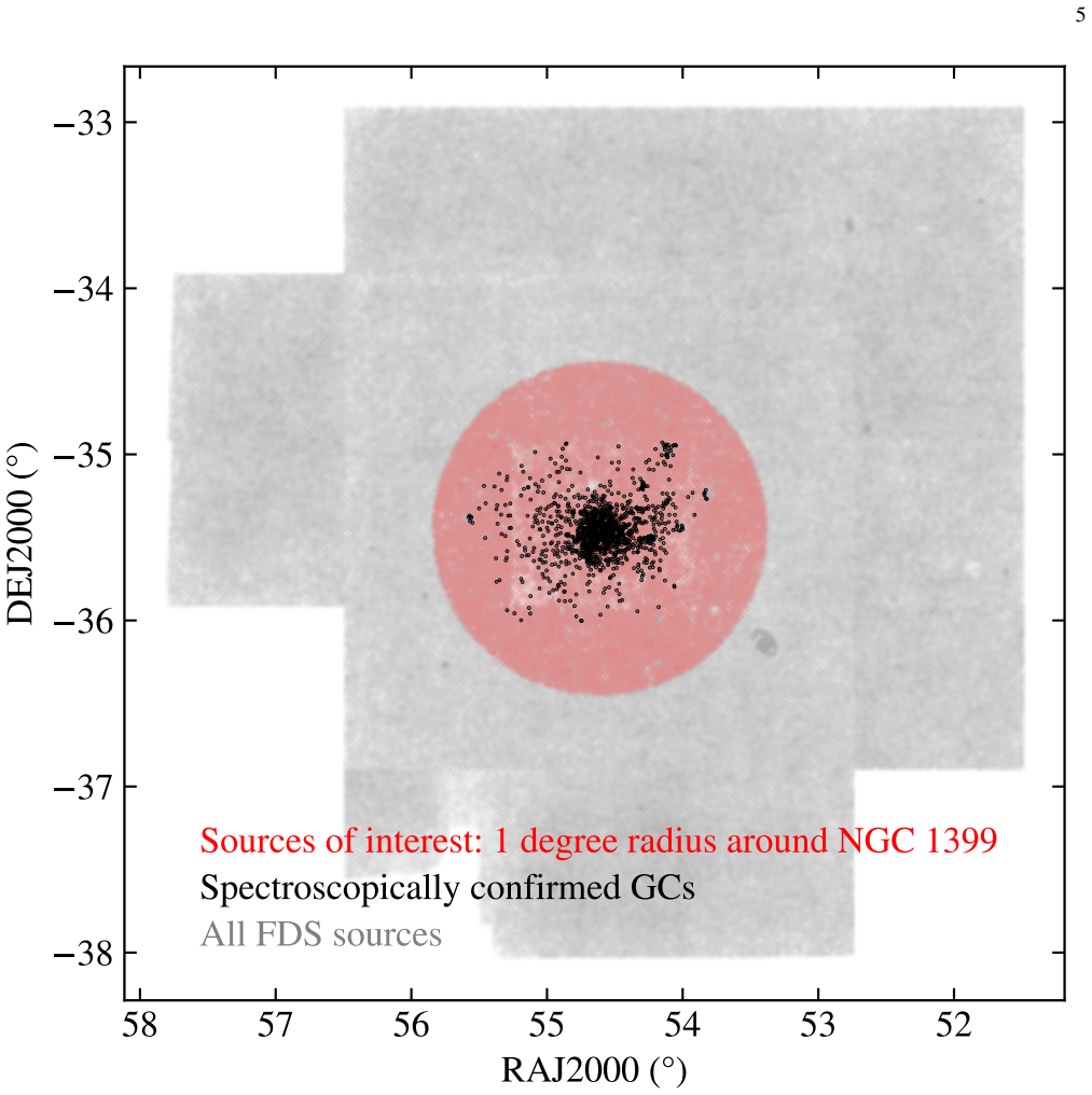
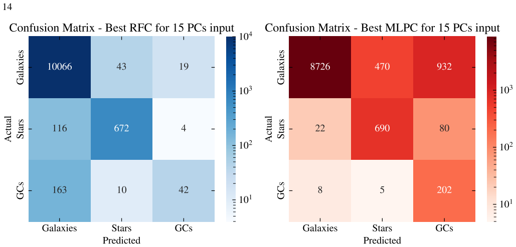
The paper assembles an LSST-like ugrizY photometric catalog of the central Fornax Cluster with labeled spectroscopically confirmed globular clusters, background galaxies, and foreground stars, and asks how well point-like globular clusters can be separated using colors alone. It finds that a random forest fed all 15 colors reaches a best precision of 57%, corresponding to roughly 43–45% contamination; feeding it the 15 principal components raises precision to 65%, corresponding to roughly 35% contamination, but recall drops to 19% — 81% of true globular clusters are missed. Non-linear auto-encoder latent coordinates do not improve on PCA or raw colors, and multi-layer perceptrons trade preci
Load-bearing premise
The foreground-star class is assumed to be almost free of real globular clusters; the paper itself says the same magnitude cut may leave 35–40% or ~10% of the GC population in that star sample, and if many GCs are mislabeled as stars, the measured contamination numbers are not a clean property of the color space.
Editorial extensions
If this is right
- For LSST-like ugrizY catalogs, color-only globular-cluster selection has a contamination floor: expect roughly 35% contamination even at best, and only with a highly incomplete (≈19% recall) candidate list.
- Principal components of the colors are a better input than the raw colors for random-forest globular-cluster selection; using 4 PCs recovers the 15-color performance, so linear compression is safe.
- Non-linear auto-encoder features do not improve globular-cluster classification over linear PCA; the information available in ugrizY colors is linearly accessible.
- Two-dimensional color-color diagrams are the weakest option, roughly doubling contamination relative to using the full high-dimensional color information.
- Reducing contamination below this floor will require augmenting colors with morphology, near-infrared, UV, or astrometric data before more complex classifiers can help.
Reading between the lines
- A testable extension: retrain the same classifiers on a version of the star sample built with space-based morphology or astrometric parallax to exclude extragalactic interlopers; if the confusion-matrix numbers change materially, the measured ~35% floor is partly a label-purity effect rather than a property of ugrizY colors.
- The same PCA-plus-random-forest recipe could be applied to the ~1000-dimensional color space of a 59-band survey such as the one the paper mentions; the authors point to PCA only as a starting point, and the extrapolation to much higher dimensional color spaces is a natural next step.
- The paper's abstract and conclusions report different contamination numbers for the 15-color case (~30% versus ~45%); a reader planning a survey should treat the higher, discussion-stage figure as the operational one, since it is the value the authors repeat in their final assessment.
- For LSST-era operations, the paper's numbers imply that photometric globular-cluster candidate lists will need to be cross-matched with space-based morphology before spectroscopic follow-up; otherwise most confirmed clusters will be missing at any acceptable purity.
Editorial analysis
A structured set of objections, weighed in public.
Referee Report
Summary. The paper assembles an LSST-like ugrizY photometric catalog of the Fornax Cluster by combining FDS u-band and DES grizY photometry, labels 1073 spectroscopically confirmed GCs plus 50,638 galaxies and 3,962 stars from DES morphology and magnitude cuts, and compares random forest and multi-layer perceptron classifiers fed with 15 colors, reduced color subsets, principal components, and auto-encoder latent coordinates. The central claim is that color-only GC selection reaches a minimum contamination of roughly 45% with raw colors, reduced to about 35% when principal components are used, while AEs give no improvement; the authors conclude that ancillary data are needed for LSST-era GC selection.
Significance. If the measurements are clean, the paper provides a useful quantitative benchmark for LSST preparation: it directly estimates the ceiling of ugrizY colors for unresolved extragalactic GC selection using a spectroscopically confirmed GC training set, and it systematically compares linear and non-linear dimensionality reductions. The qualitative conclusion that color-only selection is incomplete and contaminated, and that PCs help modestly, is plausible and broadly supported by Table 5. The paper would be strengthened by releasing code and data and by adding proper uncertainty estimates, but the empirical framing is a genuine contribution to a practical problem.
major comments (4)
- [§2.2, Eq. (2)] The GCLF paragraph is numerically self-contradictory and the purity of the 'star' class is not quantified. The text first says the mag_auto_i<=21.0 cut is at ~0.33 sigma from TOM_i~23 and leaves 35-40% of the Fornax GC population in the stellar sample, then says this fraction is ~10% for the same cut. With sigma_GCLF~1.5, a 21.0 cut sits at ~1.33 sigma, giving ~10%; a 22.5 cut gives ~37%. The star test set has 792 sources, so even a 10% hidden-GC fraction places ~80 true GCs in the 'star' class. Since precision/recall and hence the headline 35-45% contamination rates are computed against these labels, these numbers are not a clean property of the color space until the hidden-GC fraction is measured directly (e.g., from ACSFCS photometric GC candidates or a GCLF model) and label-noise sensitivity is reported.
- [§4; §3.1.2–3.2] The PCA and AE transformations appear to be fit on the entire catalog before the stratified train/test split ('We ran PCA and AEs over our LSST-like photometric catalog'). If so, the test-set features depend on test-set statistics, leaking information and biasing the comparison between raw colors and transformed inputs in favor of the PCs/LSCs. The CV protocol should fit PCA and train AEs inside each training fold only, then apply the fitted transform to the held-out fold. The paper should state explicitly where the transforms are fit and recompute Table 5 with a leakage-free protocol.
- [Table 5 and §5] The central numerical claims are quoted without uncertainty. The comparison '~45% vs ~35% contamination' corresponds to P=0.57 vs P=0.65 from a single best model per input set; there is no fold-to-fold variance, no repeated-CV error, and the best model is selected by F1 on the test set. The 4-PC result (P=0.56) is not formally distinguishable from the 15-color result (P=0.57). Report mean +/- standard deviation across CV folds (or repeated CV) and a test of significance for the PC-vs-color difference.
- [Abstract vs §5] The abstract quotes a minimum contamination of ~30% for all 15 colors, while Section 5 and the results text state ~45% for colors and ~35% for PCs. Table 5 gives P=0.57 (43% contamination) for 15 colors and P=0.65 (35%) for 15 PCs, so the abstract's 30% is not supported by the table. Align the abstract with the body, ideally after recomputing with the leakage-free protocol.
minor comments (5)
- [§4] The sentence 'On the other hand, the RFC that uses 4 LSCs as input shows a Notably, all 2D inputs yield...' is grammatically broken and should be rephrased.
- [§2.2] After correcting the GCLF arithmetic, rewrite the motivation for the 21.0 cut; the current paragraph simultaneously justifies the cut as leaving only a small fraction of GCs and as containing 35-40% of the GC population.
- [§3.1.1] The selection of the 4 and 2 most important colors uses RFC feature importance from a model trained on 15 colors; clarify whether this selection was performed inside each CV fold to avoid using test information in feature selection.
- [§5] 'Minimum contamination' should be qualified as 'minimum among the tested configurations', since no formal optimization over decision thresholds is performed.
- [Tables 6–7] The supplementary tables should adopt the same uncertainty conventions as Table 5 once they are added.
Circularity Check
No significant circularity: the central contamination/completeness claims are empirical classifier measurements on externally labeled data, not derivations from their own inputs.
full rationale
The paper's main claims—minimum contamination ~45% with colors and ~35% with principal components—are read directly from classifier precision in Table 5 (e.g., RFC 15 PCs: P=0.65, R=0.19; RFC 15 colors: P=0.57, R=0.20). These are measured confusion-matrix outputs from models trained with 5-fold stratified cross-validation on labels coming from external sources: spectroscopically confirmed GCs from Schuberth et al. (2010) and Pota et al. (2018), and DES EXTENDED_COADD morphology plus magnitude cuts for stars and galaxies. No equation defines the reported contamination/precision as equal to a fitted input, and no fitted parameter is renamed as a prediction. The PCA/AE motivation cites prior work by some of the same authors (Chies-Santos et al. 2022; de Souza et al. 2022), but the transformations themselves are standard SVD-based PCA (cited to Pedregosa et al. 2011 and Jolliffe & Cadima 2016) and standard autoencoders; those self-citations are background motivation, not the load-bearing justification for the results. The manuscript does contain an internal contradiction in Section 2.2 about the GCLF fraction of GCs inside the stellar cut (first 'roughly 35−40%', then '~10% if the cut is at 21 mag'), and the PCA/AE/feature-selection steps may have been applied before the train/test split, which would be data leakage. Both are validity and label-purity concerns that could bias the reported metrics, but neither makes the conclusion equivalent to its inputs by construction. There is no self-citation chain used as a uniqueness argument and no ansatz smuggled in via citation. The honest finding is therefore no significant circularity.
Assumptions & free parameters
free parameters (7)
- Star sample i-band magnitude cut =
19.0 ≤ mag_auto_i ≤ 21.0
- Galaxy sample i-band magnitude cut =
19.0 ≤ mag_auto_i ≤ 22.5
- Magnitude-error threshold =
0.5 mag
- Cross-match radius =
1.0 arcsec
- PCA/AE fit scope =
full catalog (before CV split)
- AE latent dimensions =
2 and 4
- Classifier hyperparameters =
randomized-search max for F1 (RFC), fixed widths for MLPC
assumptions (5)
- domain assumption The star label is clean enough: DES morphology cut plus 19.0≤i≤21.0 isolates foreground stars without major GC contamination
- domain assumption FDS ugri + DES grizY is a faithful proxy for LSST ugrizy photometry
- domain assumption Complete-case removal of missing/error-flagged sources is ignorable
- domain assumption The spectroscopically confirmed GC set is representative of the full GC population in color space
- domain assumption Fornax is representative of other galaxies' GC systems
Cite this review
Pith. "Pith review of The contribution of the color space in LSST-like photometry for the selection of extragalactic globular cluster candidates." pith.science (2026). https://pith.science/paper/BLDFO7DV
@misc{pith2026251217644,
  author       = {Pith},
  title        = {Pith review of: The contribution of the color space in LSST-like photometry for the selection of extragalactic globular cluster candidates},
  year         = {2026},
  howpublished = {\url{https://pith.science/paper/BLDFO7DV}},
  note         = {Machine review of arXiv:2512.17644}
}
abstract
Globular clusters (GCs) are excellent tracers of their host galaxies' evolutionary histories. Traditional methods for identifying GCs in galaxies rely on cuts over photometric catalogs and can yield source lists with high levels of contamination from compact background galaxies and foreground stars. In an era when large-scale sky surveys produce photometry for millions of sources, it is essential to employ flexible and scalable tools to reliably identify GCs in external galaxies. To prepare for surveys like Rubin/LSST, we need to explore practical methodological improvements and quantify the limitations inherent in the datasets. This paper investigates the selection of point-like extragalactic GCs exclusively in the $ugrizY$ color space. We use archival data to assemble an LSST-like photometric catalog for the Fornax Cluster containing labeled confirmed GCs, galaxies, and stars. From this catalog, using principal component analysis and non-linear auto-encoders (AEs), we construct inputs to random forest and multi-layer perceptron classifiers. We show that selecting GCs using all the 15 available colors can lead to a minimum contamination rate of ~30%, whereas the use of color-color diagrams may double such rate. If only the first 4 principal components of the colors are used instead, the same minimum contamination rate is achieved without increasing incompleteness. The AEs did not improve GC identification. To further reduce contamination and extract the full potential of LSST for star cluster studies, we argue for the need to augment photometric information with ancillary data (morphology from space-based missions and near-infrared photometry) before attempting to leverage more complex models.
Figures


Figures from the paper (6 more)




Reference graph
Works this paper leans on
-
[1]
Abbott, T. M. C., Adam´ow, M., Aguena, M., et al. 2021, ApJS, 255, 20, doi: 10.3847/1538-4365/ac00b3
-
[2]
2018, PASJ, 70, S8, doi: 10.1093/pasj/psx081
Aihara, H., Armstrong, R., Bickerton, S., et al. 2018, PASJ, 70, S8, doi: 10.1093/pasj/psx081
-
[3]
2019, arXiv e-prints, arXiv:1902.05569, doi: 10.48550/arXiv.1902.05569
Akeson, R., Armus, L., Bachelet, E., et al. 2019, arXiv e-prints, arXiv:1902.05569, doi: 10.48550/arXiv.1902.05569
-
[4]
Anand, G. S., Tully, R. B., Cohen, Y ., et al. 2024, ApJ, 973, 83, doi: 10.3847/1538-4357/ad64c7
-
[5]
Austin, P. C. 2011, Multivariate Behav Res., 46, 399, doi: 10.1080/00273171.2011.568786
arXiv 2011
-
[6]
2020, arXiv e-prints, arXiv:2003.05991, doi: 10.48550/arXiv.2003.05991
Bank, D., Koenigstein, N., & Giryes, R. 2020, arXiv e-prints, arXiv:2003.05991, doi: 10.48550/arXiv.2003.05991
-
[7]
Barbisan, E., Huang, J., Dage, K. C., et al. 2022, MNRAS, 514, 943, doi: 10.1093/mnras/stac1396
-
[8]
Baumgardt, H., & Hilker, M. 2018, MNRAS, 478, 1520, doi: 10.1093/mnras/sty1057 16 15 20 25 4 2 0 2 4 magFDS DES DES selected galaxies g band DES MAG_APER_5 15 20 25 r band 15.0 17.5 20.0 22.5 25.0 i band 15 20 25 4 2 0 2 4 magFDS DES DES MAG_APER_4 15 20 25 15.0 17.5 20.0 22.5 25.0 15 20 25 gFDS [mag] 4 2 0 2 4 magFDS DES DES MAG_AUTO 15 20 25 rFDS [mag] ...
Show all 73 references
-
[9]
Beasley, M. A. 2020, in Reviews in Frontiers of Modern Astrophysics; From Space Debris to Cosmology, ed. P. Kab´ath, D. Jones, & M. Skarka, 245–277, doi: 10.1007/978-3-030-38509-5 9
2020 doi
-
[10]
M., Windhorst, R
Berkheimer, J. M., Windhorst, R. A., Harris, W. E., et al. 2025, arXiv e-prints, arXiv:2508.03883, doi: 10.48550/arXiv.2508.03883
2025 doi
-
[11]
1996, A&AS, 117, 393, doi: 10.1051/aas:1996164
Bertin, E., & Arnouts, S. 1996, A&AS, 117, 393, doi: 10.1051/aas:1996164
1996 doi
-
[12]
B., Ivezi´c, ˇZ., Jones, R
Bianco, F. B., Ivezi´c, ˇZ., Jones, R. L., et al. 2022, ApJS, 258, 1, doi: 10.3847/1538-4365/ac3e72
2022 doi
- [13]
-
[14]
2001, Machine Learning, 45, 5, doi: 10.1023/A:1010933404324
Breiman, L. 2001, Machine Learning, 45, 5, doi: 10.1023/A:1010933404324
2001 doi
-
[15]
P., Romanowsky, A
Brodie, J. P., Romanowsky, A. J., Strader, J., & Forbes, D. A. 2011, AJ, 142, 199, doi: 10.1088/0004-6256/142/6/199
2011 doi
-
[16]
P., Romanowsky, A
Brodie, J. P., Romanowsky, A. J., Strader, J., et al. 2014, ApJ, 796, 52, doi: 10.1088/0004-637X/796/1/52
2014 doi
-
[17]
Burkert, A., & Forbes, D. A. 2020, AJ, 159, 56, doi: 10.3847/1538-3881/ab5b0e
2020 doi
-
[18]
A., Chies-Santos, A
Canossa-Gosteinski, M. A., Chies-Santos, A. L., Furlanetto, C., et al. 2024, MNRAS, 534, 1729, doi: 10.1093/mnras/stae2161 17 15 20 25 4 2 0 2 4 magFDS DES DES selected stars g band DES MAG_APER_5 15 20 25 r band 15.0 17.5 20.0 22.5 25.0 i band 15 20 25 4 2 0 2 4 magFDS DES DE...
2024 doi
-
[19]
2018, A&A, 611, A21, doi: 10.1051/0004-6361/201731325
Cantiello, M., Grado, A., Rejkuba, M., et al. 2018, A&A, 611, A21, doi: 10.1051/0004-6361/201731325
2018 doi
-
[20]
2020, A&A, 639, A136, doi: 10.1051/0004-6361/202038137
Cantiello, M., Venhola, A., Grado, A., et al. 2020, A&A, 639, A136, doi: 10.1051/0004-6361/202038137
2020 doi
-
[21]
Castelli, A. V . 2014, MNRAS, 442, 891, doi: 10.1093/mnras/stu876
2014 doi
-
[22]
L., Larsen, S
Chies-Santos, A. L., Larsen, S. S., Kuntschner, H., et al. 2011a, A&A, 525, A20, doi: 10.1051/0004-6361/201015683
-
[23]
L., Larsen, S
Chies-Santos, A. L., Larsen, S. S., Wehner, E. M., et al. 2011b, A&A, 525, A19, doi: 10.1051/0004-6361/201015681
-
[24]
L., de Souza, R
Chies-Santos, A. L., de Souza, R. S., Caso, J. P., et al. 2022, MNRAS, 516, 1320, doi: 10.1093/mnras/stac2002 Cˆot´e, P., Blakeslee, J. P., Ferrarese, L., et al. 2004, ApJS, 153, 223, doi: 10.1086/421490 CSST Collaboration, Gong, Y ., Miao, H., et al. 2025, arXiv e-prints, arX...
2022 doi
-
[25]
C., Zepf, S
Dage, K. C., Zepf, S. E., Thygesen, E., et al. 2020, MNRAS, 497, 596, doi: 10.1093/mnras/staa1963 de Souza, R. S., Maio, U., Biffi, V ., & Ciardi, B. 2014, MNRAS, 440, 240, doi: 10.1093/mnras/stu274 18 RFC MLPC 15 Colors (0.97, 0.99, 0.98) (0.99, 0.85, 0.92) 4 Colors (0.97, 0....
2020
-
[26]
M., Pascale, M., Frye, B., et al
Diego, J. M., Pascale, M., Frye, B., et al. 2023, A&A, 679, A159, doi: 10.1051/0004-6361/202345868
2023 doi
-
[27]
2022, A&A, 663, A81, doi: 10.1051/0004-6361/202243354
Dold, D., & Fahrion, K. 2022, A&A, 663, A81, doi: 10.1051/0004-6361/202243354
2022 doi
-
[28]
Dornan, V ., & Harris, W. E. 2025, ApJ, 988, 70, doi: 10.3847/1538-4357/ade05e
2025 doi
-
[29]
2025, arXiv e-prints, arXiv:2509.21975, doi: 10.48550/arXiv.2509.21975 Euclid Collaboration, Scaramella, R., Amiaux, J., et al
Dou, H., Li, H., Zhang, H., Yu, H., & Wang, H. 2025, arXiv e-prints, arXiv:2509.21975, doi: 10.48550/arXiv.2509.21975 Euclid Collaboration, Scaramella, R., Amiaux, J., et al. 2022, A&A, 662, A112, doi: 10.1051/0004-6361/202141938 Euclid Collaboration, V oggel, K., Lanc ¸on, A....
2025 doi
-
[30]
2020, A&A, 637, A27, doi: 10.1051/0004-6361/202037686
Fahrion, K., Lyubenova, M., Hilker, M., et al. 2020, A&A, 637, A27, doi: 10.1051/0004-6361/202037686
2020 doi
-
[31]
2012, ApJS, 200, 4, doi: 10.1088/0067-0049/200/1/4
Ferrarese, L., Cˆot´e, P., Cuillandre, J.-C., et al. 2012, ApJS, 200, 4, doi: 10.1088/0067-0049/200/1/4
2012 doi
-
[32]
A., Read, J
Forbes, D. A., Read, J. I., Gieles, M., & Collins, M. L. M. 2018, MNRAS, 481, 5592, doi: 10.1093/mnras/sty2584
2018 doi
-
[33]
2021, arXiv e-prints, arXiv:2103.04874, doi: 10.48550/arXiv.2103.04874 Gaia Collaboration, Prusti, T., de Bruijne, J
Fournier, Q., & Aloise, D. 2021, arXiv e-prints, arXiv:2103.04874, doi: 10.48550/arXiv.2103.04874 Gaia Collaboration, Prusti, T., de Bruijne, J. H. J., et al. 2016, A&A, 595, A1, doi: 10.1051/0004-6361/201629272
-
[34]
H., & Mechelli, A
Garcia-Dias, R., Vieira, S., Lopez Pinaya, W. H., & Mechelli, A. 2020, in Machine Learning, ed. A. Mechelli & S. Vieira (Academic Press), 227–247, doi: https://doi.org/10.1016/B978-0-12-815739-8.00013-4
2020 doi
-
[35]
R., & Rhode, K
Hargis, J. R., & Rhode, K. L. 2012, AJ, 144, 164, doi: 10.1088/0004-6256/144/6/164
2012 doi
-
[36]
E., Harris, G
Harris, W. E., Harris, G. L. H., & Alessi, M. 2013, ApJ, 772, 82, doi: 10.1088/0004-637X/772/2/82
2013 doi
-
[37]
E., Morningstar, W., Gnedin, O
Harris, W. E., Morningstar, W., Gnedin, O. Y ., et al. 2014, ApJ, 797, 128, doi: 10.1088/0004-637X/797/2/128
2014 doi
-
[38]
E., Imai, K., King, G., & Stuart, E
Ho, D. E., Imai, K., King, G., & Stuart, E. A. 2007, Political Analysis, 15, 199–236, doi: 10.1093/pan/mpl013
2007 doi
-
[39]
M., Ferguson, A
Howell, J. M., Ferguson, A. M. N., Larsen, S. S., et al. 2025, arXiv e-prints, arXiv:2509.10440, doi: 10.48550/arXiv.2509.10440
2025 doi
-
[40]
J., Harris, G
Hudson, M. J., Harris, G. L., & Harris, W. E. 2014, ApJL, 787, L5, doi: 10.1088/2041-8205/787/1/L5
2014 doi
-
[41]
K., Sand, D
Hughes, A. K., Sand, D. J., Seth, A., et al. 2021, ApJ, 914, 16, doi: 10.3847/1538-4357/abf63c Ivezi´c, ˇZ., Kahn, S. M., Tyson, J. A., et al. 2019, ApJ, 873, 111, doi: 10.3847/1538-4357/ab042c
2021 doi
-
[42]
T., & Cadima, J
Jolliffe, I. T., & Cadima, J. 2016, Philosophical Transactions of the Royal Society of London Series A, 374, 20150202, doi: 10.1098/rsta.2015.0202 Jord´an, A., Peng, E. W., Blakeslee, J. P., et al. 2015, ApJS, 221, 13, doi: 10.1088/0067-0049/221/1/13 19 Jord´an, A., Blakeslee,...
2016
-
[43]
2022, Nature, 602, 585, doi: 10.1038/s41586-021-04354-w
Kirsten, F., Marcote, B., Nimmo, K., et al. 2022, Nature, 602, 585, doi: 10.1038/s41586-021-04354-w
2022 doi
-
[44]
A., de Souza, R
Kuhn, M. A., de Souza, R. S., Krone-Martins, A., et al. 2021, ApJS, 254, 33, doi: 10.3847/1538-4365/abe465
2021 doi
-
[45]
S., Ferguson, A
Larsen, S. S., Ferguson, A. M. N., Howell, J. M., et al. 2025, A&A, 703, A113, doi: 10.1051/0004-6361/202554661
2025 doi
-
[46]
W., Cˆot´e, P., et al
Lim, S., Peng, E. W., Cˆot´e, P., et al. 2025, ApJS, 276, 34, doi: 10.3847/1538-4365/ad97b7
2025 doi
-
[47]
J., Kundu, A., Zepf, S
Maccarone, T. J., Kundu, A., Zepf, S. E., & Rhode, K. L. 2007, Nature, 445, 183, doi: 10.1038/nature05434
2007 doi
-
[48]
L., Jord´an, A., Cˆot´e, P., et al
Masters, K. L., Jord´an, A., Cˆot´e, P., et al. 2010, ApJ, 715, 1419, doi: 10.1088/0004-637X/715/2/1419
2010 doi
-
[49]
2024, A&A, 691, A104, doi: 10.1051/0004-6361/202451273
Mirabile, M., Cantiello, M., Lonare, P., et al. 2024, A&A, 691, A104, doi: 10.1051/0004-6361/202451273
2024 doi
-
[50]
2022, Astronomy and Computing, 39, 100555, doi: 10.1016/j.ascom.2022.100555 Mu˜noz, R
Mohammadi, M., Mutatiina, J., Saifollahi, T., & Bunte, K. 2022, Astronomy and Computing, 39, 100555, doi: 10.1016/j.ascom.2022.100555 Mu˜noz, R. P., Puzia, T. H., Lanc ¸on, A., et al. 2014, ApJS, 210, 4, doi: 10.1088/0067-0049/210/1/4
2022
-
[51]
1991, Neurocomputing, 2, 183, doi: https://doi.org/10.1016/0925-2312(91)90023-5
Murtagh, F. 1991, Neurocomputing, 2, 183, doi: https://doi.org/10.1016/0925-2312(91)90023-5
1991 doi
-
[52]
Nikutta, R., Fitzpatrick, M., Scott, A., & Weaver, B. A. 2020, Astronomy and Computing, 33, 100411, doi: 10.1016/j.ascom.2020.100411
2020
-
[53]
2000, A&AS, 143, 23, doi: 10.1051/aas:2000169
Ochsenbein, F., Bauer, P., & Marcout, J. 2000, A&AS, 143, 23, doi: 10.1051/aas:2000169
2000 doi
-
[54]
A., Coelho, P
Pacheco, T. A., Coelho, P. R. T., Martins, L. P., et al. 2025, ApJ, 992, 151, doi: 10.3847/1538-4357/adff5f
2025 doi
-
[55]
2011, Journal of Machine Learning Research, 12, 2825
Pedregosa, F., Varoquaux, G., Gramfort, A., et al. 2011, Journal of Machine Learning Research, 12, 2825
2011
-
[56]
2020, https://arxiv.org/abs/2008.12633
Peletier, R., Iodice, E., Venhola, A., et al. 2020, https://arxiv.org/abs/2008.12633
2020
-
[57]
W., Jord´an, A., Cˆot´e, P., et al
Peng, E. W., Jord´an, A., Cˆot´e, P., et al. 2006, ApJ, 639, 95, doi: 10.1086/498210
2006 doi
-
[58]
R., Hilker, M., et al
Pota, V ., Napolitano, N. R., Hilker, M., et al. 2018, MNRAS, 481, 1744, doi: 10.1093/mnras/sty2149
2018 doi
-
[59]
L., et al
Reina-Campos, M., Trujillo-Gomez, S., Pfeffer, J. L., et al. 2023, MNRAS, 521, 6368, doi: 10.1093/mnras/stad920
2023 doi
-
[60]
2012, Ap&SS, 341, 195, doi: 10.1007/s10509-012-0986-9
Rejkuba, M. 2012, Ap&SS, 341, 195, doi: 10.1007/s10509-012-0986-9
2012 doi
-
[61]
2022, MNRAS, 511, 4633, doi: 10.1093/mnras/stac328
Saifollahi, T., Zaritsky, D., Trujillo, I., et al. 2022, MNRAS, 511, 4633, doi: 10.1093/mnras/stac328
2022 doi
-
[62]
F., et al
Saifollahi, T., Janz, J., Peletier, R. F., et al. 2021, MNRAS, 504, 3580, doi: 10.1093/mnras/stab1118
2021 doi
-
[63]
2025a, A&A, 697, A10, doi: 10.1051/0004-6361/202450784
Saifollahi, T., V oggel, K., Lanc ¸on, A., et al. 2025a, A&A, 697, A10, doi: 10.1051/0004-6361/202450784
-
[64]
2025b, arXiv e-prints, arXiv:2503.16367, doi: 10.48550/arXiv.2503.16367
Saifollahi, T., Lanc ¸on, A., Cantiello, M., et al. 2025b, arXiv e-prints, arXiv:2503.16367, doi: 10.48550/arXiv.2503.16367
-
[65]
F., & Finkbeiner, D
Schlafly, E. F., & Finkbeiner, D. P. 2011, ApJ, 737, 103, doi: 10.1088/0004-637X/737/2/103
2011 doi
-
[66]
J., Finkbeiner, D
Schlegel, D. J., Finkbeiner, D. P., & Davis, M. 1998, ApJ, 500, 525, doi: 10.1086/305772
1998 doi
-
[67]
2010, A&A, 513, A52, doi: 10.1051/0004-6361/200912482
Schuberth, Y ., Richtler, T., Hilker, M., et al. 2010, A&A, 513, A52, doi: 10.1051/0004-6361/200912482
2010 doi
-
[68]
P., Forbes, D
Usher, C., Brodie, J. P., Forbes, D. A., et al. 2019, MNRAS, 490, 491, doi: 10.1093/mnras/stz2596
2019 doi
-
[69]
C., Girardi, L., et al
Usher, C., Dage, K. C., Girardi, L., et al. 2023, PASP, 135, 074201, doi: 10.1088/1538-3873/ace3f7
2023 doi
-
[70]
2021, MNRAS, 505, 5815, doi: 10.1093/mnras/stab1701
Burkert, A. 2021, MNRAS, 505, 5815, doi: 10.1093/mnras/stab1701
2021 doi
-
[71]
M., Remus, R.-S., McKenzie, M., & Forbes, D
Valenzuela, L. M., Remus, R.-S., McKenzie, M., & Forbes, D. A. 2024, A&A, 687, A104, doi: 10.1051/0004-6361/202348010 V oggel, K. T., Seth, A. C., Sand, D. J., et al. 2020, ApJ, 899, 140, doi: 10.3847/1538-4357/ab6f69
2024 doi
-
[72]
S., et al
Xu, Q., Shen, S., de Souza, R. S., et al. 2023, MNRAS, 526, 6391, doi: 10.1093/mnras/stad3181
2023 doi
-
[73]
2022, MNRAS, 513, 2609, doi: 10.1093/mnras/stac1072
Zaritsky, D. 2022, MNRAS, 513, 2609, doi: 10.1093/mnras/stac1072
2022 doi
Reviewed August 3, 2026 · model on record in the stance chip above.
Discussion (0). Continue with ORCID to comment.