REVIEW 4 major objections 5 minor 15 references
Adapting, Fast and Slow: On Few-Shot Transportability of Compositions
T0 review · 4 major / 5 minor · reviewed 2026-08-03 · deepseek-v4-flash
Pith's one-line read This paper claims that few-shot cross-domain adaptation is governed by the size of the smallest circuit of causal modules that can produce the target label, and that a structure-agnostic learner pays only a sqrt(K T*^3 log T*/n) penalty for
desk verdict Circuit transportability is a real contribution with sound proofs and an honest scope limit: the fast few-shot rates hinge on no unobserved confounding. read the letter →
The pith
A machine-rendered reading of the paper's core claim, the machinery that carries it, and where it could break.
The reading
What carries the argument
The object doing the work is the circuit, defined by a target causal model of T* variables where the label is V_{T*} and the query is P(V_{T*}|V_{1:M}). The key identity is the sequential decomposition P(v_{T*}|v_{1:M}) = Σ_{v_{M+1:T*-1}} ∏_{i=M+1}^{T*} P(v_i|pa*_i), which turns one hard transport problem into T* local module-transport problems. A discrepancy oracle Δ(i,j;i',j') says whether the mechanism and noise distribution at position i of domain j match those at position i' of domain j'; Circuit-TR pools source data for each target position licensed by Δ, learns each conditional, composes them, and marginalizes intermediates. Circuit-AD removes the need for Δ and the graphs by iteratin
What would settle it
In the binary sequential example of Section D, introduce a hidden common cause of a parent and the label while keeping the label mechanism and its noise distribution identical across source and target. If the transport claim in Theorem 2.7 holds, the target conditional remains exactly recoverable; if instead the recoverable set is an interval (as Section D argues), the no-confounding assumption is the load-bearing premise, and any fast-rate claim for confounded data fails.
Extended reading notes
Core claim
The paper's central claim is that the target predictor is transportable exactly when it can be written as a circuit—a composition of local causal mechanisms, each of which is learnable from at least one source domain—and that the speed of few-shot adaptation is controlled by the size of the smallest such circuit. Concretely, if the full causal graph and a discrepancy oracle are known, Circuit-TR composes modules from source data and predicts the target label with zero target labels, at error O(|V|^{T*}/N) when every target module is transportable. If this structural knowledge is absent, Circuit-AD enumerates all candidate circuits over all possible graphs and discrepancy partitions and picks
Load-bearing premise
The clean fast-adaptation rates assume strict positivity and no unobserved confounding in the sequential model; the paper itself shows in Section D that with hidden common causes, identical label mechanisms no longer license transport and only interval bounds remain.
Editorial extensions
If this is right
- With n target labels, the structure-agnostic learner matches the structure-informed learner up to a sqrt(K T*^3 log T*/n) penalty, so a modest number of labelled target examples can compensate for not knowing the causal graph.
- If the target label has a constant-size circuit over source modules, the learner gets near-zero-shot performance; if the minimal circuit is large (e.g., length ~ |V|^3 for GCD from max/min/subtraction), the rate is no better than target-only empirical risk minimization.
- The fast/slow threshold is quantitative: tasks with minimum circuit size L ≈ (n/K)^{1/3} are adaptable, while tasks above this threshold do not benefit from source data.
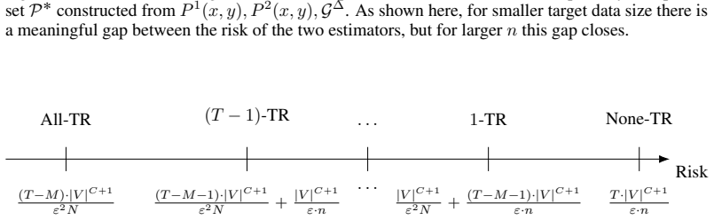
- The risk bound decomposes position by position, so each non-transportable module adds a 1/n term and intermediate regimes with partially transported circuits have predictably intermediate rates.
- Empirically, the gradient-based relaxation tracks the predicted regimes, including faster adaptation with process supervision over intermediate positions and slow adaptation when the target mechanism is not composable from the source modules.
Reading between the lines
- We infer that the selection penalty in Theorem 3.2 is not tied to causality: any learner choosing among exponentially many module compositions with a target validation set will pay sqrt(log M/n), so the rate should transfer to program synthesis and modular meta-learning with learned module libraries.
- We infer that unobserved confounding is the practical boundary: Section D shows that with a hidden common cause even identical mechanisms fail to transport, so in confounded settings the honest prediction is only an interval, and the benefit of Circuit-AD shrinks to that partial-transportation interval as n grows.
- We infer a testable extension: measuring adaptation error while varying the number of source modules available (e.g., adding a mod operator to the GCD example) should show a sharp drop at the point where the minimal circuit size crosses the (n/K)^{1/3} threshold.
- The paper's architecture learns parent matrices and mechanism clusters during pretraining; we infer that fine-tuning could be made still more sample-efficient by using intermediate supervision to estimate T*, the target circuit length, which the abstract symbolic Circuit-AD must be given in advance.
Editorial analysis
A structured set of objections, weighed in public.
Referee Report
Summary. The paper proposes a causal-transportability framework for sequential prediction. It defines module transportability, where a target conditional is learned from a source module whose mechanism and noise match the target's, and circuit transportability, where the target conditional is represented as a composition of source-learnable modules. Two algorithms are analyzed: Circuit-TR, which uses causal graphs and a discrepancy oracle, and Circuit-AD, which removes the need for this structure by searching over all candidate circuits and selecting among them with a small amount of target data. The main theoretical results are Theorem 2.7, bounding the excess risk of Circuit-TR, and Theorem 3.2, showing that the structure-agnostic Circuit-AD pays only a sqrt(K T^3 log T / n) penalty over Circuit-TR. Section 4 presents a gradient-based relaxation of the symbolic search and a synthetic experiment. The paper states that the sequential setting assumes no unobserved confounding and relegates the confounded case to Section D, where only partial-transportability bounds are obtained.
Significance. If the results hold, the paper makes a useful conceptual connection: few-shot adaptation rates are governed by the minimal circuit size of the target task relative to the source module library. The formalization of module and circuit transportability is a principled extension of causal transportability to compositional prediction, and the distinction between fast and slow adaptation regimes is well motivated. The paper has several strengths: definitions are explicit, the main theorems have self-contained proofs in the appendix, the synthetic experiments are described with reproducibility details, and Section D honestly discusses the confounded case. However, the scope of the central claims is narrower than the abstract suggests because the fast rates require the no-unobserved-confounding assumption, and one of the key proofs contains a real gap that needs to be repaired. With those fixes, the framework would be a solid contribution to the theory of domain adaptation and transfer learning.
major comments (4)
- [Section 2 (before Def. 2.5) and Section D] Theorems 2.7 and 3.2 are proved under the assumption 'there exists no unobserved confounding.' This assumption is load-bearing: the discrepancy oracle Δ(i,j;i',j') compares f and P(u_i), but without unconfoundedness equality of these objects does not imply equality of P(V_i | Pa_i) across domains. Section D itself constructs binary SCMs with identical Y mechanisms where transport fails and only bounds such as Eq. (85) are available. The central fast-adaptation rates therefore hold only in the unconfounded sequential setting. The abstract and contributions should state this limitation explicitly; alternatively, the authors should show that the rates extend to confounded cases. This is a scope limitation rather than an internal contradiction, but it is important for the paper's advertised claims.
- [Section C.4, Eqs. (55)-(65)] The proof of Theorem 2.7 as written is not valid. The Jensen-type inequality -log Σ_a ∏ µ^i_TR ≤ Σ_a -log ∏ µ^i_TR is one-sided; applying the same bound to the true µ* gives an upper bound on R_P*(µ*), not a lower bound, so the conclusion R_P*(µTR)-R_P*(µ*) ≤ Σ_i (R_P*(µ^i_TR)-R_P*(µ^i_*)) does not follow from the displayed chain. A correct proof should use the chain rule for KL divergence plus the data-processing inequality: KL(P*(v_T|v_1:M) || µTR(v_T|v_1:M)) ≤ E KL(∏ P*_i || ∏ µ^i_TR) = Σ_i E KL(P*_i || µ^i_TR). The authors need to replace the current argument with this (or an equivalent) derivation before the rate can be considered established.
- [Section 4, Proposition 4.1 / Eq. (12)] The claim that the penalized-likelihood minimizer in Eq. (12) satisfies Equations (9)-(11) is not justified as stated. The objective only depends on the observable source conditionals P^j(v_i | pa_i). If two distinct mechanisms (or two Markov-equivalent parent graphs) induce the same conditional distribution, source data alone cannot distinguish them, so the exact discrepancy oracle Φ and the true parent matrices are not identifiable without additional assumptions. The proof in Section C.6 asserts that a suitable λ enforces these properties, but it does not provide identification conditions or control the penalty/optimization error. If this proposition is meant to justify the practical algorithm, that is acceptable as a heuristic, but the proposition should be stated with explicit assumptions or weakened.
- [Section 4.2, Proposition 4.2] The proof of Proposition 4.2 (Section C.7) analyzes a discretized version of the fine-tuning procedure: binary parent matrices, binary transport indicators, and a grid search over that finite set. The actual implemented method in Section 4.2 solves the continuous optimization in Eq. (16) for s_i ∈ [0,1] and performs a gradient-based search; it does not globally search the finite grid used in the proof. Therefore the statement R_P*(µft) = O(R_P*(µAD)) is not established for the actual two-stage procedure. The authors should either analyze the implemented objective, or state explicitly that the proposition applies only to the discretized idealization and not to the reported experiments.
minor comments (5)
- [Abstract / Section 2] The no-unobserved-confounding assumption should be mentioned in the abstract and in the contributions list, not only in the body before Definition 2.5. Currently the abstract promises 'zero-shot/few-shot' guarantees without this caveat.
- [Theorem 2.7 vs. Eq. (68)] The 'otherwise' case in Theorem 2.7 states O(|V|^{M+1}/(ϵ n)), but the refined bound in Eq. (68) depends on the number of non-transported modules and on c = max|Pa_i^∗|. The theorem statement should be aligned with the refined bound, or the coarser statement should be derived from it.
- [Section C.5, Eq. (72)-(73)] The bound on log|H| is written as O(K T^3 log T), but the displayed expression gives O(K T^2 log T). The T^3 bound is safe as an overestimate, but the notation should be made precise to avoid confusion.
- [Example 3.3, Eq. (8)] The statement 'n = Ω(|V|^3)' omits the log factor that appears in Eq. (8); the threshold should be n = Ω(|V|^3 log |V|), unless the log is absorbed in the Ω notation with a stated convention.
- [Algorithm 2, line 3] The notation D^{j'}[Y: V_{i'}, X:1:c: Pa^{j'}_{i'}] should clarify how ordered parent tuples are aligned when the source and target parent sets use different orderings. The mechanism-sharing notion in Definition 2.5 should specify whether the compared functions are on the ordered tuples as given.
Circularity Check
No significant circularity: the main risk bounds are derived from stated structural assumptions and standard ERM/finite-class arguments, not by defining the target in terms of the predictor.
full rationale
I walked the paper's derivation chain. The main results (Theorem 2.7 and Theorem 3.2) are proved from explicit probabilistic conditions: strict positivity, no unobserved confounding in the sequential setting, the discrepancy oracle, and finite discrete variables. Theorem 2.7's proof (Appendix C.4) decomposes the risk of the composed circuit into per-position risks, uses Jensen/concavity, and then applies standard ERM excess-risk bounds (Lemma C.2, Corollary C.3, Lemma C.4). The fit is not renamed as a prediction: each module is learned from pooled source data only when the discrepancy oracle reports mechanism equality, and the no-confounding assumption is what licenses the equality of conditionals. Theorem 3.2's proof (Appendix C.5) is an oracle inequality: Algorithm 3 enumerates all compatible structures, so the structure-informed circuit-TR solution is one candidate in the class H; the held-out target data selects from H, and uniform convergence over H gives the sqrt(K T^3 log T / n) penalty. This is not circular, because mu_AD is not defined from mu_TR's value; it is defined by empirical risk minimization over a class that includes mu_TR as a member. The inclusion of the true structure is a completeness/coverage property of the enumeration, and the bound is a standard finite-class selection guarantee. The paper's reliance on the authors' prior transportability work is contextual: Pearl/Bareinboim transportability, partial transportability (Jalaldoust et al., 2024), and completeness results are cited for background or for the confounded-case limitation in Section D. These citations are not used to derive the central no-confounding fast/slow rates, and Section D itself explicitly constructs binary SCMs to demonstrate the confounder obstruction, providing independent support for the limitation. The honest limitation in Section D does reduce the scope of the advertised fast-adaptation result to unconfounded settings, but that is a stated assumption of Theorem 2.7, not a circular step. No equation in the paper fits the target result into the inputs by construction, and no fitted parameter is renamed as a prediction. I therefore find no significant circularity.
Assumptions & free parameters
free parameters (3)
- target circuit size T*
- pretraining penalty lambda =
unspecified 'small enough'
- sharp-softmax temperature tau =
0.1
assumptions (6)
- standard math Recursive SCMs with no cyclic dependencies (Definition 1.1)
- domain assumption Strict positivity: P^j(x,y) > epsilon for all j and a known constant epsilon
- domain assumption No unobserved confounding in the sequential setting
- domain assumption Known causal order V1 < ... < VT and shared finite vocabulary
- domain assumption Exact discrepancy oracle and causal diagrams available to Circuit-TR
- standard math Finite-class uniform convergence bounds from VC theory
Cite this review
Pith. "Pith review of Adapting, Fast and Slow: On Few-Shot Transportability of Compositions." pith.science (2026). https://pith.science/paper/SWCT7VWD
@misc{pith2026251222777,
  author       = {Pith},
  title        = {Pith review of: Adapting, Fast and Slow: On Few-Shot Transportability of Compositions},
  year         = {2026},
  howpublished = {\url{https://pith.science/paper/SWCT7VWD}},
  note         = {Machine review of arXiv:2512.22777}
}
read the original abstract
Generalization across domains requires stable structure that links the source and target distributions. Building on causal transportability theory, we study a sequential prediction setting in which the target predictor can be represented as a circuit composed of causal mechanisms that are learnable from source data. We introduce two classes of transportability. Module transportability captures the atomic case, where the target predictor is given by a mechanism learnable from a single source domain. Circuit transportability generalizes this idea to target predictors obtained by composing several modules learned from source data, enabling zero-shot prediction even when no source mechanism directly predicts the target label. We study these classes of circuits under increasingly relaxed assumptions. First, we provide conditions under which the relevant circuits can be learned from source data alone, given causal knowledge about the source and target domains. We then relax these structural assumptions by allowing limited data from the target domain. In particular, we develop a supervised domain adaptation scheme that learns circuits without requiring explicit causal structure. The resulting few-shot guarantees tie the achievable error to the size of the smallest target circuit composable from modules learned from source data. Finally, we propose a gradient-based relaxation of the symbolic circuit search and evaluate it empirically, showing that it qualitatively tracks the predicted regimes of fast adaptation -- with and without process supervision over intermediate positions -- and slow adaptation when no source mechanism matches.
Figures


Figures from the paper (6 more)




Reference graph
Works this paper leans on
-
[1]
The target mechanism indicatorΦ ˚ :rTsÑrd θsrcs
-
[2]
The target parent matrixA ˚Pr0,1s TˆT
-
[3]
The target-only predictorsµ ˚ ipvi|v 1:i´1q
-
[4]
XÐU X‘U XY YÐpX‘U XYq‘U Y M2 : $ ’’’’’& ’’’’’% P 2pUq: $ & % UX„Bernp0.9q UY „Bernp0.05q UXY „Bernp0.95q F 2 :
The transport indicatorss 1, ..., sT Pr0,1s Once the pretrained parameters θsrc satisfy Equations (9) to (11), consider the following values for the parameters of fine-tuning stage: Let A˚ encode the true causal diagram G˚, and for the transported conditionals P˚pvi |pa ˚ iq we set si “1 , and Φ˚piq “Φpi1, j1q for somepi1, j1q which satisfies ∆pi,˚;i 1, j...
2011
-
[6]
A selectedcausal function(e.g., add, subtract, multiply)
-
[7]
One or moreparent tokensfrom earlier positions in the sequence (i.e., positionsăi) INPUT REPRESENTATION AND POSITIONAL ENCODING Input sequences: Sequences of integer token IDs fromV“t0,1, . . . ,9u. Positional encoding( PositionalEncoding class): Each token at positionpi, jqwhere i is the sequence position andjis the domain ID is mapped to a dense vector ...
-
[8]
The h-dimensional embedding of each token is passed through a linear projection to |F| dimensions
-
[9]
Layer normalization is applied: LayerNormpLinearpembeddingqq
Show all 15 references
-
[10]
Thechoice of operation is contextual based on the token’s embedding, but themeaningof each operation is universal across domains
Softmax produces a probability distribution: softmaxpLayerNormpLinearpembeddingqqq Universality: This module’s parameters are shared across all domains and positions. Thechoice of operation is contextual based on the token’s embedding, but themeaningof each operation is univer...
-
[11]
Output: For each domain j, a list of C attention weight matrices pB, T, Tqrepresenting parent selection distributions
Causal masking: Standard causal attention masking ensures token at position i only attends to positionsăi 3.Sharp softmax:A j,h“softmaxpS j,h{τqwhereτ“0.1 4.First position handling: Weights for position0are zeroed as it has no parents The temperature τ“0.1 makes the softmax si...
-
[12]
Operator indicators operator_indicatorsr:, p,:sform the first part of the feature vector
-
[13]
, C´1u: WeightedParentValueh,p“A j,hr:, p,:s¨sequences_onehot (95) wherejis the domain of positioni
For each parent headhPt0, . . . , C´1u: WeightedParentValueh,p“A j,hr:, p,:s¨sequences_onehot (95) wherejis the domain of positioni. This produces apB,|V|qvector for each parent head
-
[14]
TheseCvectors are concatenated after the operator indicators Feature dimension:|F|`pCˆ|V|qwhere|F|is the number of operations and|V|“10. CONDITIONALMLPFOR PREDICTION TheEfficientConditionalMLPclass predicts the next token’s probability distribution based on the combined featur...
-
[15]
Hidden layers: Stack of linear layers (rÑr ) with ReLU activations, dropout, and residual connections 3.Output layer: Linear layer fromrto|V|“10 Output: Logits of shapepB, T,|V|qfor next-token prediction. TRAINING AND FINE-TUNING PROTOCOL Pre-training (source domains): The ent...
-
[2007]
tπ1, π2, ..., πKu that entail the source distributions P src“tP 1px, yq, P2px, yq, . . . , PKpx, yqu. Let n“|D ˚| and N“|D j| for all jPrKs , and suppose N
URL https://proceedings.neurips.cc/paper_files/paper/2007/ file/42e77b63637ab381e8be5f8318cc28a2-Paper.pdf. John Blitzer, Sham Kakade, and Dean Foster. Domain adaptation with coupled subspaces. In Proceedings of the Fourteenth International Conference on Artificial Intelligenc...
2007 arXiv
Reviewed August 3, 2026 · model on record in the stance chip above.
Discussion (0). Continue with ORCID to comment.