REVIEW 4 major objections 4 minor 1 cited by
Noise-Driven Exploration and Transient Freezing Select Flat Minima in Stochastic Gradient Descent
T0 review · 4 major / 4 minor · reviewed 2026-08-03 · deepseek-v4-flash
Pith's one-line read SGD's preference for flat minima comes from a transient freezing transition, not a static bias.
desk verdict The transient-freezing mechanism is new and plausible; the continuation experiment is the best evidence, but the quantitative theory rests on free constants and a loss-threshold proxy. read the letter →
The pith
A machine-rendered reading of the paper's core claim, the machinery that carries it, and where it could break.
The reading
What carries the argument
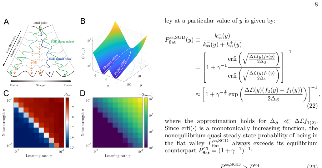
The central object is a two-dimensional bifurcating-valley loss landscape in which one valley is flatter than the other, and the dynamics is a discrete-time Langevin equation with noise covariance proportional to the local Hessian. The key identity is the effective potential L_eff(x,y) derived from the non-equilibrium steady state, which adds a control-dependent correction term that favors the flatter valley. The freezing point y_freeze, set by comparing Kramers' escape rates to the longitudinal drift rate, is what converts the steady-state bias into a transient selection. Together, these yield the closed-form probability P_tr,flat that increases with noise strength.
What would settle it
Train a neural network with a noise schedule that is initially large and then abruptly dropped to zero (or to a very small value) before the empirically observed freezing time. If the final solution remains in the sharp valley despite the early high-noise phase, the transient freezing mechanism would be contradicted. Alternatively, measure the freezing time as a function of noise and check whether the probability of landing in a flat valley decreases when noise is increased at fixed y (as the static steady-state would predict) in a controlled landscape where y is fixed.
Extended reading notes
Core claim
The core discovery is that SGD selects flat minima through a transient freezing mechanism. Using a minimal two-valley model with Hessian-proportional noise, the authors show that anisotropic noise creates an effective loss landscape that deepens the flat valley and raises the sharp one, biasing exploration. However, the final outcome is not set by the steady-state distribution alone: as the loss decreases, valley flatness and barrier heights grow, suppressing inter-valley transitions. The freezing point y_freeze increases with noise strength, so stronger noise (larger learning rate or smaller batch size) prolongs the exploratory phase. The transient probability of ending in the flatter valle
Load-bearing premise
The two-dimensional bifurcating-valley landscape with Hessian-proportional noise is assumed to faithfully represent the essential dynamics of high-dimensional neural-network loss landscapes, an assertion that is argued but not directly measured in real networks.
Editorial extensions
If this is right
- If correct, the early transient phase of training determines which valley is selected, so learning-rate and batch-size schedules should be viewed as tools for regulating the duration of exploration before freezing.
- The framework implies that any noise anisotropy aligned with local curvature can bias selection toward flatter regions, not just the specific SGD noise model.
- The freezing mechanism predicts that delaying freezing, e.g., by adaptively increasing noise early in training, should improve generalization without sacrificing convergence.
- The theory distinguishes SGD's bias from dynamic-instability explanations, showing a preference for flat minima can arise even when all valleys are dynamically stable.
- The model predicts that the flatness contrast γ between valleys amplifies the noise-driven bias, so landscapes with more heterogeneous curvature should show stronger flat-minimum selection.
Reading between the lines
- The freezing mechanism suggests a concrete experimental test: interrupting training with a noise burst after freezing should not change the final valley, whereas a similar burst before freezing should redirect the trajectory to a different basin.
- The two-valley model may extend to many-valley landscapes as a directed, biased random walk that is progressively frozen; one could test whether the final valley distribution matches the transient probability formula with an effective γ.
- The paper's claim that freezing time grows with noise implies that batch-size schedules that gradually increase batch size (decreasing noise) could be used to freeze early and preserve sharp minima if desired, or to delay freezing and encourage flatter solutions.
- If Hessian-proportional noise is essential, then optimizers using other noise structures (e.g., isotropic or momentum-based) should show weaker flat-minimum selection, which can be tested empirically.
Editorial analysis
A structured set of objections, weighed in public.
Referee Report
Summary. The paper studies the early transient dynamics of stochastic gradient descent (SGD) and proposes a mechanism for its preference for flat minima. Empirically, on a 1000-sample MNIST subset with a two-hidden-layer MLP, the authors show that increasing SGD noise (smaller batch size or larger learning rate) leads to more diverse final solutions, higher test accuracy, and flatter minima (Fig. 2). They define the freezing time t_freeze as the first iteration at which the training loss drops below a threshold L_c=0.1 (Eq. 7) and report that larger noise increases this time (Fig. 3). A continuation experiment, in which training is branched to full-batch GD at different times, suggests that valley switching occurs almost exclusively before t_freeze (Fig. 4). To explain these observations, the authors construct a two-dimensional bifurcating-valley loss landscape with Hessian-proportional Gaussian noise (Eqs. 8-15). Simulations of this toy model reproduce the qualitative trends in flat-valley probability and freezing time. The theoretical analysis derives an effective potential that biases dynamics toward the flatter valley (Eqs. 19-20), and a transient-freezing approximation (Eqs. 24-26) predicts that stronger noise delays freezing and increases the probability of selecting the flatter valley. The paper frames this as a nonequilibrium mechanism distinct from previously proposed dynamic-instability explanations.
Significance. If the transient-freezing mechanism is correct, it would provide a unified and physically appealing account of SGD's flat-minima bias, with concrete implications for learning-rate and batch-size schedules. The continuation-training experiment is a genuine methodological contribution, and the public code availability is a strength. The toy-model analysis is clear and the qualitative match with the empirical trends is encouraging. However, the current evidence is suggestive rather than conclusive: the central analytic prediction Eq. (26) contains free constants that are not fixed or measured, the loss-based proxy for freezing is only validated for one hyperparameter setting, and the toy model builds in the Hessian-proportional noise assumption that is the ultimate source of the reported bias. The extension to high-dimensional neural networks rests on an asserted low-dimensional reduction. These issues leave the central mechanism plausible but not quantitatively established.
major comments (4)
- [§II.G and Appendix A.4, Eq. (26)] The final transient probability P_tr,SGD_flat depends on ε and Φ, which are introduced as arbitrary constants: ε is a small freezing-criterion constant and Φ absorbs other model parameters via an upper-bound approximation. The derivation therefore makes a concrete prediction for the noise-dependence only up to two undetermined parameters. As written, the claim that P_flat increases with ΔS follows from the functional form (ΔS)^{1-γ} for any γ>1, and the constants cannot be checked or falsified from data. To make Eq. (26) a testable prediction, the authors should either fix ε and Φ from independent measurements in the toy model (e.g., from simulated escape rates), or report the predicted P_flat versus ΔS curve against simulations without free rescaling.
- [§II.C, §II.D, Eq. (7) and Fig. 4] The central quantity t_freeze is defined as the first iteration where the training loss crosses L_c=0.1, not as the last iteration at which the trajectory switches valleys. The continuation experiment validates the equivalence between this loss-based t_freeze and the cessation of valley switching for only one hyperparameter setting (B=50, η=0.05). The subsequent claim that 'increasing SGD noise delays freezing' (Fig. 3B,C) is therefore based on a proxy whose equivalence is not established across the (η,B) heatmap. If the loss threshold is crossed earlier or later for reasons unrelated to barrier crossing—for example, changes in loss scale or gradient magnitude—the measured delay would not establish a delayed valley-freezing transition. The authors should validate the proxy for at least low- and high-noise settings, or measure valley-switching times directly.
- [§II.E, Eq. (15)] The toy model assumes the SGD noise covariance is proportional to the Hessian, Σ=2σH. The effective-potential bias (Eqs. 19-20) follows directly from this assumption: with Σ∝H, the SGD correction term is negative in the flatter valley and positive in the sharper valley by construction. Thus the model demonstrates a consequence of Hessian-proportional noise, but does not provide evidence that real SGD noise indeed has this property, nor does it quantify the effect size in real networks. The cited empirical references [17,18,23] are not substantiated by measurements in this manuscript. I recommend either reporting direct evidence of the noise-Hessian relationship for the MLP used here (e.g., alignment of the noise covariance and Hessian eigenvectors) or explicitly framing this as an unvalidated but motivating assumption.
- [§III, penultimate paragraph] The generalization of the toy model to high-dimensional networks rests on the assertion that 'optimization in deep learning is constrained to a highly degenerate, effectively low-dimensional submanifold of parameter space' with one downhill direction and one valley-selection direction. This reduction is asserted rather than derived or empirically demonstrated. Without evidence that the trained MLP's dynamics are effectively two-dimensional in the relevant sense, the connection between the toy model and the real-network experiments remains an assumption. I suggest adding a dimensionality analysis of the SGD trajectory subspace (e.g., participation ratio of the PCA components) or softening the claim substantially.
minor comments (4)
- [§II.C, Eq. (7)] The choice L_c=0.1 and its sensitivity are only discussed in the Supplemental Material; a sentence in the main text stating the range of thresholds for which the qualitative conclusions hold would improve readability.
- [§II.E, text near Eq. (8)] Typo: 'shaper valleys' should be 'sharper valleys' in the list of empirical features.
- [§II.F, Eq. (21)-(22)] The notation ΔL is introduced in Eq. (11) but used again in Eq. (21) without restating the definition; adding a pointer to Eq. (11) would avoid confusion.
- [Fig. 5] The definition of η⟨t_freeze⟩ for the toy model (last valley-switching iteration) appears only in the Supplemental Material; it should be stated in the main text since it differs from the empirical definition of t_freeze.
Circularity Check
No significant circularity; the freezing mechanism is derived from the model equations, and self-citations are supporting rather than load-bearing.
full rationale
The empirical findings are direct measurements: clustered valleys, barrier-height correlations, noise-dependent flatness and accuracy, and continuation experiments showing valley switching. The two-valley model is introduced as a minimal mechanism with an explicit Hessian-proportional noise ansatz (Eq. 15: Sigma=2sigma H), and the paper explicitly describes the landscape as 'constructed' to contain flat/sharp valleys (Eq. 10 and gamma>1). This is a modeling choice, not a disguised fit of the empirical outcome. The steady-state calculation (Eq. 22) is derived in Appendix A from the model, and it actually shows the opposite noise dependence at fixed y: increasing Delta_S weakens the flat-valley preference. The central claim is therefore the transient-freezing correction (Eqs. 24-26), which follows from the derived escape-rate/drift balance and the analytic expression for y_freeze, rather than being inserted by hand. The undetermined constants epsilon and Phi in Eq. 25/26 limit quantitative falsifiability, but that is a modeling weakness, not circularity. Self-citations [14,19,23] exist, but the key noise-Hessian assumption is also supported by external references [17,18,21], and the effective-potential result is rederived independently in Appendix A. Thus no load-bearing step reduces to its own input by construction.
Assumptions & free parameters
free parameters (4)
- ε (freezing criterion constant)
- Φ (effective constant absorbing model parameters) =
upper-bound approximation in Eq. A33
- flatness ratio γ=(x1/x2)^2 =
>1; x1=0.8 in simulations
- toy landscape geometry {x1,x2,y_b,y_f,f0,x0,L_d,y_d} =
f0=x0=1.0, x1=0.8 in main text; others in SM Table S1
assumptions (5)
- domain assumption SGD gradient-noise covariance is proportional to the Hessian: Σ(θ)=2σH(θ)
- domain assumption Adiabatic/quasi-steady-state timescale separation τ_x≪τ_y
- domain assumption Rare-escape Kramers regime ΔS≪ΔL f1(2)
- ad hoc to paper Freezing criterion k^-_ss≈ε|Pdot/P| with small constant ε
- ad hoc to paper Real high-dimensional loss landscapes reduce to the two effective degrees of freedom (x,y) of the toy model
Cite this review
Pith. "Pith review of Noise-Driven Exploration and Transient Freezing Select Flat Minima in Stochastic Gradient Descent." pith.science (2026). https://pith.science/paper/3XCVGKOF
@misc{pith2026260110962,
  author       = {Pith},
  title        = {Pith review of: Noise-Driven Exploration and Transient Freezing Select Flat Minima in Stochastic Gradient Descent},
  year         = {2026},
  howpublished = {\url{https://pith.science/paper/3XCVGKOF}},
  note         = {Machine review of arXiv:2601.10962}
}
read the original abstract
Stochastic gradient descent (SGD) is central to deep learning, yet the dynamical origin of its preference for flatter, more generalizable solutions remains unclear. Here, by analyzing SGD learning dynamics, we identify a nonequilibrium mechanism that governs solution selection during training. Numerical experiments reveal a transient exploratory phase in which SGD trajectories repeatedly escape sharp valleys and migrate toward flatter regions of the loss landscape before becoming confined to a final basin. Using a tractable physical model, we show that SGD noise reshapes the loss landscape into an effective potential that preferentially stabilizes flat solutions. We further uncover a transient freezing mechanism: as training progresses, the flattening landscape suppresses transitions between competing valleys. Stronger SGD noise delays this freezing transition, prolonging the exploratory phase and thereby increasing the probability of convergence to flatter minima. Together, these results provide a unified physical framework connecting learning dynamics, loss-landscape geometry, and generalization, and suggest guiding principles for the design of more effective optimization algorithms.
Figures


Figures from the paper (3 more)


Forward citations
Cited by 1 Pith paper
-
On the Superlinear Relationship between SGD Noise Covariance and Loss Landscape Curvature
SGD noise covariance is claimed to follow the second moment of per-sample Hessians, giving a superlinear power law C_ii ∝ H_ii^γ with 1 ≤ γ ≤ 2.
Reference graph
Works this paper leans on
-
[1]
Continuous-time dynamics and F okker-Planck equation We analyze the continuous-time limit of the discrete SGD update rule: θt+1 =θ t −η∇L(θ t)−ηξ t,(A1) where the gradient noise satisfiesE[ξ t] = 0 and Cov[ξt] = Σ(θt). By interpreting the learning rateηas the dis- cretization time step ∆t, the process converges to the fol- lowing stochastic differential e...
-
[2]
The dynamics in thex-direction are governed by the local curvatureκ x ≡∂ 2 xL
Non-equilibrium steady state and effective loss Our derivation relies on the adiabatic approximation, the validity of which depends on a distinct separation of timescales between the fast transverse relaxation within the valleys (x-direction) and the slow longitudinal drift (y-direction). The dynamics in thex-direction are governed by the local curvatureκ...
-
[3]
Based on the Fokker- Planck equation, the MFPT from the sharp valley mini- mum (x⋆
Kramers’ escape rates and steady-state convergence probability We quantify inter-valley transitions using the Mean First Passage Time (MFPT) [42]. Based on the Fokker- Planck equation, the MFPT from the sharp valley mini- mum (x⋆
-
[4]
to the barrier (x= 0), denotedτ s→f , is: τs→f = 1 D− 11 Z 0 x⋆ 2 dx′e L(x′ ) D− 11 Z x′ −∞ dx′′e − L(x′′) D− 11 .(A19) Similarly, for the transition from the flat valley minimum (x⋆
-
[5]
to the sharp side (τ f→s ): τf→s = 1 D+ 11 Z x⋆ 1 0 dx′e L(x′ ) D+ 11 Z +∞ x′ dx′′e − L(x′′ ) D+ 11 .(A20) We apply Kramers’ approximation, assuming rare es- cape events. This regime holds when the noise amplitude is small relative to the barrier height (D ± 11 ≪∆L), sat- isfying: ∆S ≪ 1 2 x1(2)y y+y b 2 .(A21) In this limit, the double integrals decouple...
-
[6]
Asyincreases, the escape ratesk ± decrease ex- ponentially
The freezing mechanism and transient dynamics approximation The final solution selection is governed by the com- petition between inter-valley diffusion and longitudinal drift. Asyincreases, the escape ratesk ± decrease ex- ponentially. The system ”freezes” when the transition timescale exceeds the drift timescale. The final probabil- ity is approximated ...
-
[7]
LeCun, Y
Y. LeCun, Y. Bengio, and G. Hinton, Deep learning, Na- ture521, 436 (2015)
2015
-
[8]
Levine and Y
H. Levine and Y. Tu, Machine learning meets physics: A two-way street, Proceedings of the National Academy of Sciences121, e2403580121 (2024)
2024
Show all 48 references
-
[9]
C. Liu, L. Zhu, and M. Belkin, Loss landscapes and op- timization in over-parameterized non-linear systems and neural networks, Applied and Computational Harmonic Analysis59, 85 (2022)
2022
-
[10]
R. Sun, D. Li, S. Liang, T. Ding, and R. Srikant, The Global Landscape of Neural Networks: An Overview, IEEE Signal Processing Magazine37, 95 (2020), arXiv:2007.01429 [cs, math, stat]
2020 arXiv
-
[11]
Zhang, Y
Y. Zhang, Y. Li, Z. Zhang, T. L. Null, and Z.-Q. J. Xu, Embedding Principle: A Hierarchical Structure of Loss Landscape of Deep Neural Networks, Journal of Machine Learning1, 60 (2022)
2022
-
[12]
Choromanska, M
A. Choromanska, M. Henaff, M. Mathieu, G. B. Arous, and Y. LeCun, The loss surfaces of multilayer networks, inInternational Conference on Artificial Intelligence and Statistics (AISTATS), Vol. 38 (JMLR, 2015) pp. 192– 204
2015
-
[13]
W. R. Huang, Z. Emam, M. Goldblum, L. Fowl, J. K. Terry, F. Huang, and T. Goldstein, Understanding gen- eralization through visualizations, inICBINB@NeurIPS, Proceedings of Machine Learning Research, Vol. 137 (PMLR, 2020) pp. 87–97
2020
-
[14]
Hochreiter and J
S. Hochreiter and J. Schmidhuber, Flat minima, Neural Computation9, 1 (1997)
1997
-
[15]
H. Li, Z. Xu, G. Taylor, C. Studer, and T. Goldstein, Visualizing the loss landscape of neural nets, inNeurIPS (2018) pp. 6391–6401
2018
-
[16]
Jastrzebski, Z
S. Jastrzebski, Z. Kenton, D. Arpit, N. Ballas, A. Fis- cher, Y. Bengio, and A. Storkey, Three factors influencing minima in SGD, inInternational Conference on Artificial Neural Networks (ICANN)(Springer, 2018) pp. 169–180
2018
-
[17]
L. Wu, C. Ma, and W. E, How SGD selects the global minima in over-parameterized learning: A dynamical sta- bility perspective, inNeurIPS(2018) pp. 8289–8298
2018
-
[18]
N. S. Keskar, D. Mudigere, J. Nocedal, M. Smelyan- skiy, and P. T. P. Tang, On large-batch training for deep learning: Generalization gap and sharp minima, inICLR (2017)
2017
-
[19]
S. Chen, S. Recanatesi, and E. Shea-Brown, A simple connection from loss flatness to compressed represen- tations in neural networks, arXiv:2310.01770 (2024), arXiv:2310.01770 [cs]
2024
-
[20]
Y. Feng, W. Zhang, and Y. Tu, Activity–weight du- ality in feed-forward neural networks reveals two co- determinants for generalization, Nature Machine Intel- ligence5, 908 (2023)
2023
-
[21]
Robbins and S
H. Robbins and S. Monro, A Stochastic Approximation Method, The Annals of Mathematical Statistics22, 400 (1951), 2236626
1951
-
[22]
Bottou, Large-scale machine learning with stochastic gradient descent, inCOMPSTAT(Physica-Verlag, 2010) pp
L. Bottou, Large-scale machine learning with stochastic gradient descent, inCOMPSTAT(Physica-Verlag, 2010) pp. 177–186
2010
-
[23]
Xie, Q.-Y
Z. Xie, Q.-Y. Tang, M. Sun, and P. Li, On the overlooked structure of stochastic gradients, inNeurIPS(2023)
2023
-
[24]
J. Z. HaoChen, C. Wei, J. Lee, and T. Ma, Shape Mat- ters: Understanding the Implicit Bias of the Noise Co- variance, inProceedings of Thirty Fourth Conference on Learning Theory(PMLR, 2021) pp. 2315–2357
2021
-
[25]
Feng and Y
Y. Feng and Y. Tu, The inverse variance–flatness rela- tion in stochastic gradient descent is critical for finding flat minima, Proceedings of the National Academy of Sci- ences118, e2015617118 (2021)
2021
-
[26]
Z. Zhu, J. Wu, B. Yu, L. Wu, and J. Ma, The anisotropic noise in stochastic gradient descent: Its behavior of es- caping from sharp minima and regularization effects, inICML, Proceedings of Machine Learning Research, Vol. 97 (PMLR, 2019) pp. 7654–7663
2019
-
[27]
Z. Xie, I. Sato, and M. Sugiyama, A diffusion theory for deep learning dynamics: Stochastic gradient descent exponentially favors flat minima, inICLR(2021)
2021
-
[28]
X. Li, Q. Gu, Y. Zhou, T. Chen, and A. Banerjee, Hes- sian based analysis of SGD for deep nets: Dynamics and generalization, inSDM(SIAM, 2020) pp. 190–198
2020
-
[29]
N. Yang, C. Tang, and Y. Tu, Stochastic Gradient De- scent Introduces an Effective Landscape-Dependent Reg- ularization Favoring Flat Solutions, Physical Review Let- ters130, 237101 (2023)
2023
-
[30]
Chaudhari, A
P. Chaudhari, A. Choromanska, S. Soatto, Y. Le- Cun, C. Baldassi, C. Borgs, J. Chayes, L. Sagun, and R. Zecchina, Entropy-SGD: Biasing gradient descent into wide valleys, Journal of Statistical Mechanics: Theory and Experiment2019, 124018 (2019)
2019
-
[31]
Wei and D
M. Wei and D. J. Schwab, How noise affects the Hes- sian spectrum in overparameterized neural networks, arXiv:1910.00195 (2019), arXiv:1910.00195
1910 arXiv
- [32]
- [33]
-
[34]
Feng and Y
Y. Feng and Y. Tu, Phases of learning dynamics in arti- ficial neural networks in the absence or presence of mis- labeled data, Machine Learning: Science and Technology 2, 043001 (2021)
2021
-
[35]
D. S. Kalra and M. Barkeshli, Phase diagram of early training dynamics in deep neural networks: Effect of the learning rate, depth, and width, inNeurIPS(2023)
2023
-
[36]
Jastrzebski, M
S. Jastrzebski, M. Szymczak, S. Fort, D. Arpit, J. Tabor, K. Cho, and K. J. Geras, The break-even point on op- timization trajectories of deep neural networks, inICLR (2020)
2020
-
[37]
Frankle and M
J. Frankle and M. Carbin, The lottery ticket hypothe- sis: Finding sparse, trainable neural networks, inICLR (2019)
2019
-
[38]
Ghorbani, S
B. Ghorbani, S. Krishnan, and Y. Xiao, An investiga- tion into neural net optimization via hessian eigenvalue density, inICML, Proceedings of Machine Learning Re- search, Vol. 97 (PMLR, 2019) pp. 2232–2241
2019
-
[39]
Sagun, U
L. Sagun, U. Evci, V. U. G¨ uney, Y. N. Dauphin, and L. Bottou, Empirical analysis of the hessian of over-parametrized neural networks, inICLR (Workshop) (2018)
2018
-
[40]
Waddington, The strategy of the genes (1957)
CH. Waddington, The strategy of the genes (1957)
1957
-
[41]
Kitano, Towards a theory of biological robustness, 15 Molecular Systems Biology3, 137 (2007)
H. Kitano, Towards a theory of biological robustness, 15 Molecular Systems Biology3, 137 (2007)
2007
-
[42]
J. Wang, K. Zhang, L. Xu, and E. Wang, Quantifying the Waddington landscape and biological paths for devel- opment and differentiation, Proceedings of the National Academy of Sciences108, 8257 (2011)
2011
-
[43]
Pujadas and A
E. Pujadas and A. P. Feinberg, Regulated Noise in the Epigenetic Landscape of Development and Disease, Cell 148, 1123 (2012)
2012
-
[44]
J. E. Ferrell, Bistability, Bifurcations, and Waddington’s Epigenetic Landscape, Current Biology22, R458 (2012)
2012
-
[45]
Fort and S
S. Fort and S. Jastrzebski, Large scale structure of neural network loss landscapes, inNeurIPS(2019) pp. 6706– 6714
2019
-
[46]
Garipov, P
T. Garipov, P. Izmailov, D. Podoprikhin, D. P. Vetrov, and A. G. Wilson, Loss surfaces, mode connectivity, and fast ensembling of dnns, inNeurIPS(2018) pp. 8803– 8812
2018
-
[47]
Q. Li, C. Tai, and E. Weinan, Stochastic modified equa- tions and adaptive stochastic gradient algorithms, inIn- ternational Conference on Machine Learning(PMLR,
-
[48]
Gardiner,Stochastic Methods, Vol
C. Gardiner,Stochastic Methods, Vol. 4 (Springer Berlin, 2009)
2009
Reviewed August 3, 2026 · model on record in the stance chip above.
Discussion (0). Continue with ORCID to comment.