Recognition: 2 theorem links
· Lean TheoremTidal Deformation Bounds and Perturbation Transfer in Bounded Curvature Spacetimes
Pith reviewed 2026-05-15 21:29 UTC · model grok-4.3
The pith
A global bound on tidal forces along free-fall paths implies a strict upper limit on accumulated geodesic deviation controlled by τ* = λ_max^{-1/2} and a critical wavenumber separating adiabatic from non-adiabatic perturbation transfer.
A machine-rendered reading of the paper's core claim, the machinery that carries it, and where it could break.
Core claim
Given an invariant bound λ_max ≤ λ_bound on the electric Riemann eigenvalues E_ij along freely falling worldlines, the accumulated geodesic deviation through any bounded curvature interior is rigorously upper-bounded by a scale controlled by τ* ≡ λ_max^{-1/2}. There also exists a critical wavenumber k* ~ τ*^{-1} that separates adiabatic from non-adiabatic perturbation transfer, with Bogoliubov coefficients exponentially suppressed for k τ* ≫ 1. Both results hold independently of further metric details once the tidal bound and a mild timescale condition on the curvature-driven effective potential are satisfied.
What carries the argument
The global upper bound λ_max on the electric Riemann eigenvalues E_ij measured by freely falling observers, which defines the single characteristic timescale τ* = λ_max^{-1/2} that governs both accumulated deviation and mode transfer.
If this is right
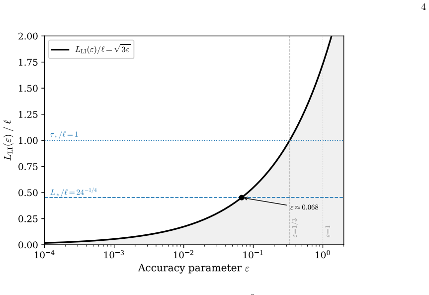
- The accuracy-dependent size of the local-inertial domain scales as the square root of the desired accuracy times τ*.
- In conformally flat four-dimensional cores the ratio of τ* to the curvature radius L* equals 24 to the power one-fourth.
- High-wavenumber modes experience exponential suppression of their Bogoliubov coefficients when crossing the bounded-curvature epoch.
- The same tidal bound controls deviation accumulation for any metric that respects it, without reference to other curvature components.
- Numerical integration in the extremal Hayward geometry confirms that the predicted scales remain accurate.
Where Pith is reading between the lines
- The same bounding argument could be applied to other curvature scalars to obtain resolution scales for additional observables.
- These results suggest that effective descriptions of fields or particles near strong gravity can remain valid farther into the high-curvature regime than metric-specific analyses indicate.
- Departures from conformal flatness quantified by the Weyl-to-Kretschmann ratio provide a direct way to estimate corrections in more general spacetimes.
Load-bearing premise
The electric Riemann eigenvalues remain bounded above by λ_max along every freely falling worldline throughout the region of interest.
What would settle it
A calculation or measurement of geodesic deviation that exceeds the derived upper bound inside a spacetime whose measured electric Riemann eigenvalues never surpass the assumed λ_max would directly contradict the central claim.
Figures


read the original abstract
We derive two model-independent results for spacetimes with globally bounded tidal fields. These are operational resolution scales of the local-inertial approximation and tidal dynamics; no spacetime discreteness is implied. Given an invariant bound $\lambda_{\max}\le\lambda_{\rm bound}$ on the electric Riemann eigenvalues $E_{ij}\equiv R_{\hat{0}i\hat{0}j}$ along freely falling worldlines, we prove (i)~a rigorous upper bound on accumulated geodesic deviation through any bounded curvature interior, controlled by $\tau_*\equiv\lambda_{\max}^{-1/2}$, and (ii)~the existence of a critical wavenumber $k_*\sim\tau_*^{-1}$ separating adiabatic from non-adiabatic perturbation transfer through high-curvature epochs, with Bogoliubov coefficients exponentially suppressed for $k\,\tau_*\gg 1$. Both results depend only on the tidal bound (and, for mode transfer, on a mild timescale assumption for the curvature-driven effective potential) and are otherwise insensitive to metric details. For preparation, we collect the standard operational consequences of bounded curvature, including the accuracy-dependent local-inertial domain $L_{\rm LI}(\varepsilon)\sim\sqrt{\varepsilon}\, \lambda_{\max}^{-1/2}$ and, for conformally flat cores in four dimensions, the benchmark ratio $\tau_*/L_*=24^{1/4}$ with $L_*\equiv K_{\max}^{-1/4}$. We quantify the robustness of this coefficient under departures from maximal symmetry via the Weyl-to-Kretschmann ratio $\epsilon_C$. The general framework is validated numerically in the extremal Hayward geometry.
Editorial analysis
A structured set of objections, weighed in public.
Referee Report
Summary. The paper derives two model-independent results for spacetimes with globally bounded tidal fields: given an invariant bound λ_max on the electric Riemann eigenvalues E_ij along freely falling worldlines, it proves (i) a rigorous upper bound on accumulated geodesic deviation controlled by τ* ≡ λ_max^{-1/2}, and (ii) the existence of a critical wavenumber k* ~ τ*^{-1} separating adiabatic from non-adiabatic perturbation transfer, with Bogoliubov coefficients exponentially suppressed for k τ* ≫ 1. Both results depend only on the tidal bound (plus a mild timescale assumption on the curvature-driven effective potential for the mode-transfer case). The manuscript also collects operational consequences of bounded curvature, including the local-inertial domain L_LI(ε) ~ √ε λ_max^{-1/2}, a benchmark ratio τ*/L* = 24^{1/4} for conformally flat 4D cores, and its robustness under Weyl-to-Kretschmann ratio ε_C, with numerical validation in the extremal Hayward geometry.
Significance. If the central claims hold, the results supply metric-insensitive operational scales for the validity of the local-inertial approximation and for mode evolution across high-curvature epochs. These could be useful in regular black-hole models, numerical relativity, and QFT in curved spacetime. The derivations rest on standard linear-ODE comparison theorems and adiabatic/WKB estimates, which are correctly identified as load-bearing; the single-geometry numerical check provides supporting evidence but is not the primary justification.
major comments (2)
- [derivation of accumulated geodesic deviation bound] The geodesic-deviation bound (abstract and the section deriving result (i)) follows from the standard comparison theorem applied to D²ξ^i/Dτ² = −E^i_j ξ^j with ||E|| ≤ λ_max. The manuscript should state the explicit comparison solution (e.g., ||ξ(τ)|| ≤ f(τ/τ*) with initial conditions ξ(0), ξ'(0) specified) and any error term arising from the time dependence of E_ij; without this, the precise functional form of the accumulated-deviation bound remains implicit.
- [derivation of perturbation-transfer result] For the mode-transfer result (abstract and the section deriving result (ii)), the mild timescale assumption on the curvature-induced effective potential is invoked to obtain the adiabaticity criterion k ≫ 1/τ*. This assumption should be written as an explicit quantitative condition (e.g., |dV_eff/dτ| / k^3 ≪ 1 or equivalent) so that its domain of applicability can be checked in concrete spacetimes; the current phrasing leaves the threshold for “mild” unspecified.
minor comments (3)
- [numerical validation section] The numerical validation is performed only for the extremal Hayward geometry; a brief remark on why this geometry is representative (or a second example) would strengthen the supporting evidence without altering the model-independent claims.
- [preparation section on operational consequences] The benchmark ratio τ*/L* = 24^{1/4} and its dependence on ε_C are stated for conformally flat cores; a short table or plot of the ratio versus ε_C would make the robustness quantification easier to read.
- [throughout] Notation: the hats on frame indices (E_{ij} ≡ R_{0̂i0̂j}) are used inconsistently in a few places; a single global convention would improve clarity.
Simulated Author's Rebuttal
We thank the referee for the careful reading and constructive comments. We address each major comment below and will incorporate the suggested clarifications to improve the explicitness of the derivations.
read point-by-point responses
-
Referee: [derivation of accumulated geodesic deviation bound] The geodesic-deviation bound (abstract and the section deriving result (i)) follows from the standard comparison theorem applied to D²ξ^i/Dτ² = −E^i_j ξ^j with ||E|| ≤ λ_max. The manuscript should state the explicit comparison solution (e.g., ||ξ(τ)|| ≤ f(τ/τ*) with initial conditions ξ(0), ξ'(0) specified) and any error term arising from the time dependence of E_ij; without this, the precise functional form of the accumulated-deviation bound remains implicit.
Authors: We agree that an explicit statement of the comparison solution will enhance clarity. In the revised manuscript we will add the precise form obtained from the standard Sturm comparison theorem: for the geodesic deviation equation with ||E|| ≤ λ_max, the worst-case (defocusing) bound is ||ξ(τ)|| ≤ ||ξ(0)|| cosh(τ/τ_*) + τ_* ||ξ'(0)|| sinh(τ/τ_*), where the initial conditions ξ(0) and ξ'(0) are taken at entry to the bounded-curvature region. Because the comparison theorem supplies a rigorous envelope for any time-dependent E satisfying the bound, no additional error term arises from the time dependence of E_ij. revision: yes
-
Referee: [derivation of perturbation-transfer result] For the mode-transfer result (abstract and the section deriving result (ii)), the mild timescale assumption on the curvature-induced effective potential is invoked to obtain the adiabaticity criterion k ≫ 1/τ*. This assumption should be written as an explicit quantitative condition (e.g., |dV_eff/dτ| / k^3 ≪ 1 or equivalent) so that its domain of applicability can be checked in concrete spacetimes; the current phrasing leaves the threshold for “mild” unspecified.
Authors: We accept the suggestion to quantify the assumption. In the revised manuscript we will state the mild-timescale condition explicitly as |dV_eff/dτ| ≪ k^3 (where V_eff is the curvature-induced effective potential), which directly yields the adiabaticity criterion k ≫ τ_*^{-1} and permits immediate verification in any concrete spacetime by evaluating the derivative of V_eff. revision: yes
Circularity Check
No significant circularity; derivation self-contained from input tidal bound
full rationale
The paper takes the invariant bound λ_max on electric Riemann eigenvalues E_ij along freely falling worldlines as an external input and derives the geodesic-deviation bound via standard comparison theorems applied to the linear ODE D²ξ^i/Dτ² = −E^i_j ξ^j with ||E|| ≤ λ_max, yielding control by τ* = λ_max^{-1/2}. The critical wavenumber k* and Bogoliubov suppression follow from the usual WKB/adiabatic theorem estimates once the mild timescale assumption on the curvature-driven effective potential is imposed. No equation reduces the claimed results to a self-definition, a fitted parameter, or a load-bearing self-citation; the framework is validated numerically in Hayward geometry as independent confirmation rather than part of the derivation.
Axiom & Free-Parameter Ledger
axioms (1)
- domain assumption Tidal fields (electric Riemann eigenvalues E_ij) are globally bounded by some λ_bound along all freely falling worldlines
Lean theorems connected to this paper
-
IndisputableMonolith/CostdAlembert_cosh_solution_aczel echoes?
echoesECHOES: this paper passage has the same mathematical shape or conceptual pattern as the Recognition theorem, but is not a direct formal dependency.
If |λ(τ)| ≤ λ_max ... then |ξ(Δτ)| ≤ |ξ(0)| cosh(Δτ/τ*) + τ* |˙ξ(0)| sinh(Δτ/τ*), τ* ≡ λ_max^{-1/2}. The proof uses the Sturm comparison theorem ... ¨¯ξ = λ_max ¯ξ
-
IndisputableMonolith/Foundation/AlphaCoordinateFixationcostAlphaLog_high_calibrated_iff echoes?
echoesECHOES: this paper passage has the same mathematical shape or conceptual pattern as the Recognition theorem, but is not a direct formal dependency.
A_k ≲ α λ_max^{3/2} / (k^2 + λ_max)^{3/2}; modes with k τ* ≫ 1 propagate adiabatically with exponentially suppressed Bogoliubov mixing
What do these tags mean?
- matches
- The paper's claim is directly supported by a theorem in the formal canon.
- supports
- The theorem supports part of the paper's argument, but the paper may add assumptions or extra steps.
- extends
- The paper goes beyond the formal theorem; the theorem is a base layer rather than the whole result.
- uses
- The paper appears to rely on the theorem as machinery.
- contradicts
- The paper's claim conflicts with a theorem or certificate in the canon.
- unclear
- Pith found a possible connection, but the passage is too broad, indirect, or ambiguous to say the theorem truly supports the claim.
Reference graph
Works this paper leans on
-
[1]
Setup and Metric Components The Hayward metric is given by equation (3) with the metric function f(r) = 1− 2M r2 r3 + 2M ℓ2 .(A1) For computational clarity, we introduce the dimensionless variables x≡ r ℓ , m≡ M ℓ ,(A2) so that f(x) = 1− 2mx2 x3 + 2m.(A3) The non-vanishing metric components in coordinates (t, r, θ, ϕ) are gtt =−f(r), g rr =f(r) −1, g θθ =...
-
[2]
Riemann Tensor Components For a static, spherically symmetric metric, the independent non-vanishing components of the Riemann tensor (in an orthonormal frame) are: Rˆt ˆrˆtˆr=− 1 2 f ′′(r),(A5) Rˆt ˆθˆtˆθ =R ˆt ˆϕˆtˆϕ =− f ′(r) 2r ,(A6) Rˆr ˆθˆrˆθ =R ˆr ˆϕˆrˆϕ =− f ′(r) 2r ,(A7) R ˆθ ˆϕˆθ ˆϕ = 1−f(r) r2 .(A8) Here, primes denote derivatives with respect t...
-
[3]
Derivatives of the Metric Function From equation (A1), direct differentiation yields the first derivative: f ′(r) = 2M r(r3 −4M ℓ 2) (r3 + 2M ℓ2)2 .(A9) Differentiating again and simplifying gives the second derivative: f ′′(r) = −4M(r 6 −14M ℓ 2r3 + 4M2ℓ4) (r3 + 2M ℓ2)3 .(A10)
-
[4]
Behavior at the Origin Taking limits asr→0: f(0) = 1, f ′(0) = 0, f ′′(0) =− 2 ℓ2 .(A11) Thus, nearr= 0: f(r)≈1− r2 ℓ2 +O(r 4),(A12) confirming the de Sitter form with effective cosmological constant Λ eff = 3/ℓ2
-
[5]
Kretschmann Scalar and Monotonicity The Kretschmann scalar is defined asK=R µνρσ Rµνρσ. For our metric: K= (f ′′)2 + 4(f ′)2 r2 + 4(1−f) 2 r4 .(A13) Using equations (A9) and (A10) in equation (A13), the Kretschmann scalar can be written in closed form as: K(r) = 48M2 r12 −8M ℓ 2r9 + 72M2ℓ4r6 −16M 3ℓ6r3 + 32M4ℓ8 (r3 + 2M ℓ2)6 .(A14) 13 As cross-checks, equ...
-
[6]
Weyl-squared scalar for static spherically symmetric metrics For a static, spherically symmetric line element with lapse functionf(r) (equation (A1)), the six independent orthonormal-frame Riemann components reduce to three independent functions,[34] A ≡R ˆ0ˆ1ˆ0ˆ1 = 1 2 f ′′,(B1) B ≡R ˆ0ˆ2ˆ0ˆ2 =R ˆ0ˆ3ˆ0ˆ3 = f ′ 2r ,(B2) F ≡R ˆ2ˆ3ˆ2ˆ3 = 1−f r2 ,(B3) withR ...
-
[7]
Closed-form expressions for the Hayward metric For the Hayward lapse, usingD≡r 3 + 2M ℓ2 for brevity, one obtains A −2B − F=− 6M r3(r3 −4M ℓ 2) D3 ,(B7) and therefore C2(r) = 48M 2r6 (r3 −4M ℓ 2)2 (r3 + 2M ℓ2)6 .(B8) a. Asymptotic checks. •Core (r→0):The prefactorr 6 ensuresC 2(0) = 0, confirming that the de Sitter core is conformally flat. •Schwarzschild...
-
[8]
The anisotropy parameterϵ C(r) The dimensionless Weyl-to-Kretschmann ratio introduced in equation (21), ϵ2 C(r)≡ C2(r) K(r) ,0≤ϵ C ≤1,(B9) is most conveniently expressed in terms of the dimensionless radial variabley≡r 3/(M ℓ2): ϵ2 C(y) = y2 (y−4) 2 y4 −8y 3 + 72y2 −16y+ 32 .(B10) This function satisfiesϵ C(0) = 0 (maximally symmetric core) andϵ C(4) = 0 ...
-
[9]
Tidal eigenvalues and operational ratio away from the core For the Hayward metric, the two distinct tidal eigenvalues (in units ofℓ −2) are λ1 ℓ2 = −2(y2 −14y+ 4) (y+ 2) 3 , λ 2 ℓ2 = y−4 (y+ 2) 2 ,(B11) 15 TABLE I. Anisotropy parameterϵ C, tidal eigenvalues, and operational ratioτ ∗/L∗ as functions ofy=r 3/(M ℓ2) for the Hayward metric. The maximally symm...
-
[10]
Penrose, Gravitational collapse and space-time singularities, Phys
R. Penrose, Gravitational collapse and space-time singularities, Phys. Rev. Lett.14, 57 (1965)
work page 1965
-
[11]
S. W. Hawking and R. Penrose, The singularities of gravitational collapse and cosmology, Proc. Roy. Soc. Lond. A314, 529 (1970)
work page 1970
-
[12]
Kiefer,Quantum Gravity, 2nd ed
C. Kiefer,Quantum Gravity, 2nd ed. (Oxford University Press, 2007)
work page 2007
-
[13]
Rovelli,Quantum Gravity(Cambridge University Press, 2004)
C. Rovelli,Quantum Gravity(Cambridge University Press, 2004)
work page 2004
-
[14]
Minimal Length Scale Scenarios for Quantum Gravity
S. Hossenfelder, Minimal length scale scenarios for quantum gravity, Living Rev. Rel.16, 2 (2013), arXiv:1203.6191 [hep-th]
work page internal anchor Pith review Pith/arXiv arXiv 2013
-
[15]
M. A. Markov, Limiting density of matter as a universal law of nature, JETP Lett.36, 266 (1982)
work page 1982
-
[16]
V. F. Mukhanov and R. H. Brandenberger, A nonsingular universe, Phys. Rev. Lett.68, 1969 (1992)
work page 1969
-
[17]
R. H. Brandenberger, V. F. Mukhanov, and A. Sornborger, Cosmological theory without singularities, Phys. Rev. D48, 1629 (1993), arXiv:gr-qc/9303001
work page internal anchor Pith review Pith/arXiv arXiv 1993
- [18]
- [19]
-
[20]
V. P. Frolov and A. Zelnikov, Spherically symmetric black holes in the limiting curvature theory of gravity, Phys. Rev. D 105, 024041 (2022), arXiv:2111.12846 [gr-qc]. 16 0 10 20 30 40 50 60 0.0 0.2 0.4 0.6 0.8 1.0ϵC ≡ √ C 2/K y=4 → 1 y ϵmax C =1/3 λ1=0 ϵC(y) 0 10 20 30 40 50 60 y ≡ r3/(Mℓ 2) 1.0 1.5 2.0 2.5 3.0 3.5τ ∗ /L ∗ = K 1/4/|λmax|1/2 ±10% τ ∗ /L ∗...
-
[21]
J. M. Bardeen, Non-singular general-relativistic gravitational collapse, inProc. Int. Conf. GR5(Tbilisi, 1968) p. 174
work page 1968
- [22]
-
[23]
S. Ansoldi, Spherical black holes with regular center: A review of existing models including a recent realization with Gaussian sources (2008) arXiv:0802.0330 [gr-qc]
work page internal anchor Pith review Pith/arXiv arXiv 2008
-
[24]
V. P. Frolov, Notes on nonsingular models of black holes, Phys. Rev. D94, 104056 (2016), arXiv:1609.01758 [gr-qc]
work page internal anchor Pith review Pith/arXiv arXiv 2016
-
[25]
C. W. Misner, K. S. Thorne, and J. A. Wheeler,Gravitation(W. H. Freeman, San Francisco, 1973)
work page 1973
-
[26]
R. M. Wald,General Relativity(University of Chicago Press, 1984)
work page 1984
-
[27]
Hartman,Ordinary Differential Equations(Wiley, New York, 1964) reprinted by SIAM, 2002
P. Hartman,Ordinary Differential Equations(Wiley, New York, 1964) reprinted by SIAM, 2002. See Ch. XI, Theorem 3.1
work page 1964
-
[28]
M. Drobczyk, A density-responsive scalar-field framework for singularity regularization and dynamical dark energy, Clas- sical and Quantum Gravity42, 225016 (2025)
work page 2025
-
[29]
A Generalized Uncertainty Principle in Quantum Gravity
M. Maggiore, A generalized uncertainty principle in quantum gravity, Phys. Lett. B304, 65 (1993), arXiv:hep-th/9301067
work page internal anchor Pith review Pith/arXiv arXiv 1993
-
[30]
Generalized Uncertainty Principle in Quantum Gravity from Micro-Black Hole Gedanken Experiment
F. Scardigli, Generalized uncertainty principle in quantum gravity from micro-black hole gedanken experiment, Phys. Lett. B452, 39 (1999), arXiv:hep-th/9904025
work page internal anchor Pith review Pith/arXiv arXiv 1999
- [31]
-
[32]
Renormalization group improved black hole spacetimes
A. Bonanno and M. Reuter, Renormalization group improved black hole spacetimes, Phys. Rev. D62, 043008 (2000), arXiv:hep-th/0002196
work page internal anchor Pith review Pith/arXiv arXiv 2000
-
[33]
M. Reuter and F. Saueressig, Quantum Einstein gravity, New J. Phys.14, 055022 (2012), arXiv:1202.2274 [hep-th]
work page internal anchor Pith review Pith/arXiv arXiv 2012
-
[34]
Noncommutative Black Holes, The Final Appeal To Quantum Gravity: A Review
P. Nicolini, Noncommutative black holes, the final appeal to quantum gravity: A review, Int. J. Mod. Phys. A24, 1229 17 (2009), arXiv:0807.1939 [hep-th]
work page internal anchor Pith review Pith/arXiv arXiv 2009
-
[35]
N. D. Birrell and P. C. W. Davies,Quantum Fields in Curved Space(Cambridge University Press, 1982)
work page 1982
-
[36]
E. Poisson and W. Israel, Internal structure of black holes, Phys. Rev. D41, 1796 (1990)
work page 1990
-
[37]
On the viability of regular black holes
R. Carballo-Rubio, F. Di Filippo, S. Liberati, C. Pacilio, and M. Visser, On the viability of regular black holes, JHEP07, 023, arXiv:1805.02675 [gr-qc]
work page internal anchor Pith review Pith/arXiv arXiv
-
[38]
Is the gravitational-wave ringdown a probe of the event horizon?
V. Cardoso, E. Franzin, and P. Pani, Is the gravitational-wave ringdown a probe of the event horizon?, Phys. Rev. Lett. 116, 171101 (2016), erratum: Phys. Rev. Lett.117, 089902 (2016), arXiv:1602.07309 [gr-qc]
work page internal anchor Pith review Pith/arXiv arXiv 2016
-
[39]
Relativistic theory of tidal Love numbers
T. Binnington and E. Poisson, Relativistic theory of tidal Love numbers, Phys. Rev. D80, 084018 (2009), arXiv:0906.1366 [gr-qc]
work page internal anchor Pith review Pith/arXiv arXiv 2009
-
[40]
H. Salecker and E. P. Wigner, Quantum limitations of the measurement of space-time distances, Phys. Rev.109, 571 (1958)
work page 1958
-
[41]
Universal decoherence due to gravitational time dilation
I. Pikovski, M. Zych, F. Costa, and ˇC. Brukner, Universal decoherence due to gravitational time dilation, Nature Phys. 11, 668 (2015), arXiv:1311.1095 [quant-ph]
work page internal anchor Pith review Pith/arXiv arXiv 2015
-
[42]
M. Drobczyk, Code for: Tidal deformation bounds and perturbation transfer in bounded curvature spacetimes (2026)
work page 2026
-
[43]
These are all-lower-index orthonormal-frame components. The sign ofRˆ0ˆ1ˆ0ˆ1 differs from the mixed-index expressionR ˆ0 ˆ1ˆ0ˆ1 = −f ′′/2 commonly quoted in the literature by a factorg ˆ0ˆ0 =−1
discussion (0)
Sign in with ORCID, Apple, or X to comment. Anyone can read and Pith papers without signing in.