Geodesics from Quantum Field Theory: A Case Study in AdS
Pith reviewed 2026-05-10 19:57 UTC · model grok-4.3
The pith
The stress tensor expectation value of a localized quantum state traces a geodesic in any curved spacetime.
A machine-rendered reading of the paper's core claim, the machinery that carries it, and where it could break.
Core claim
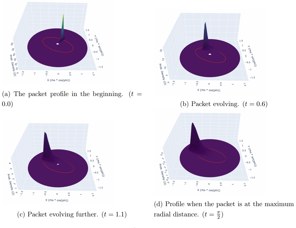
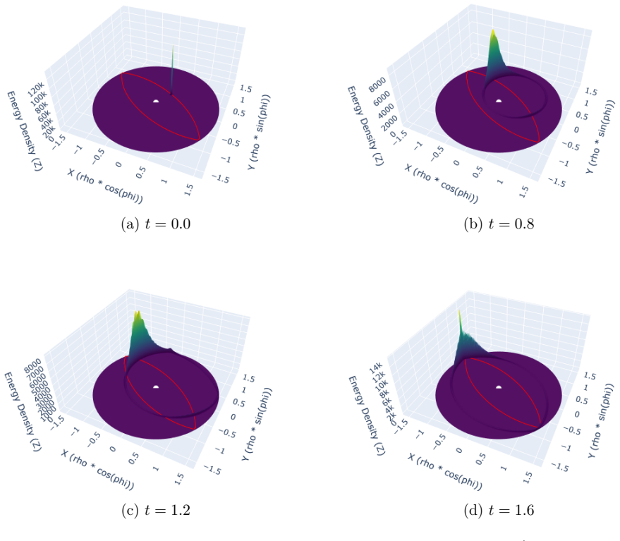
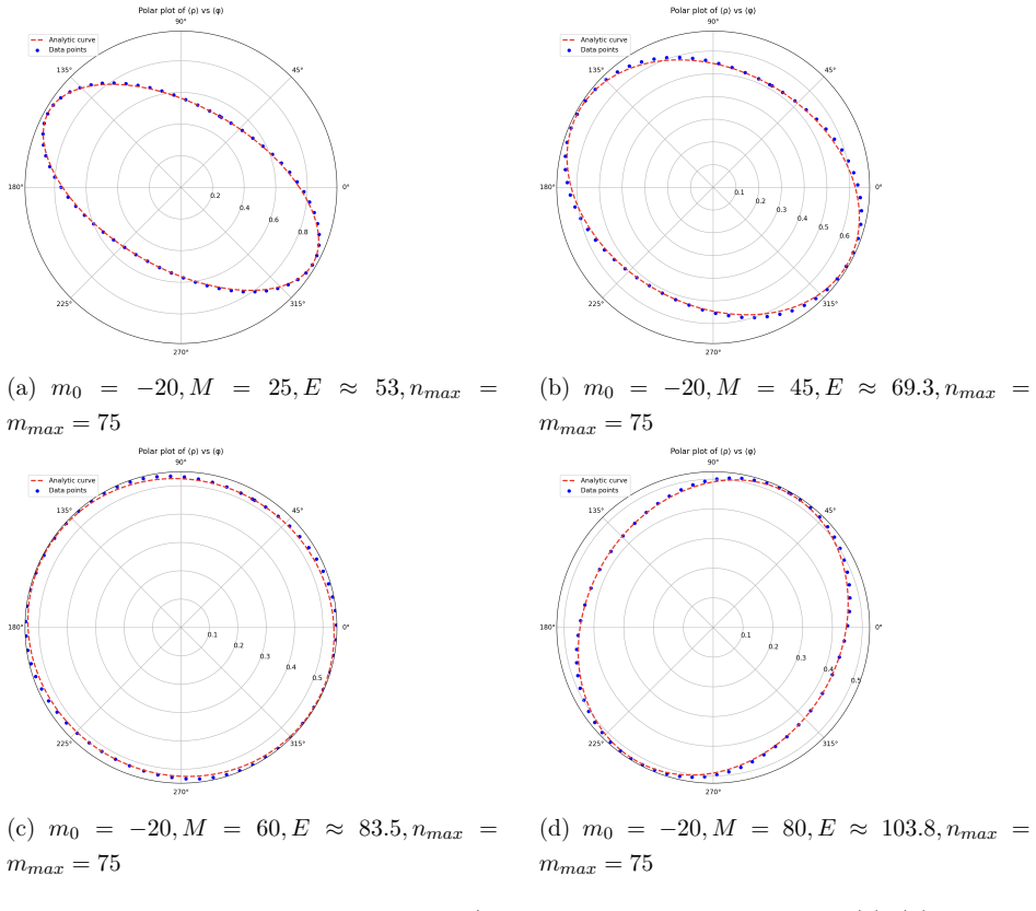
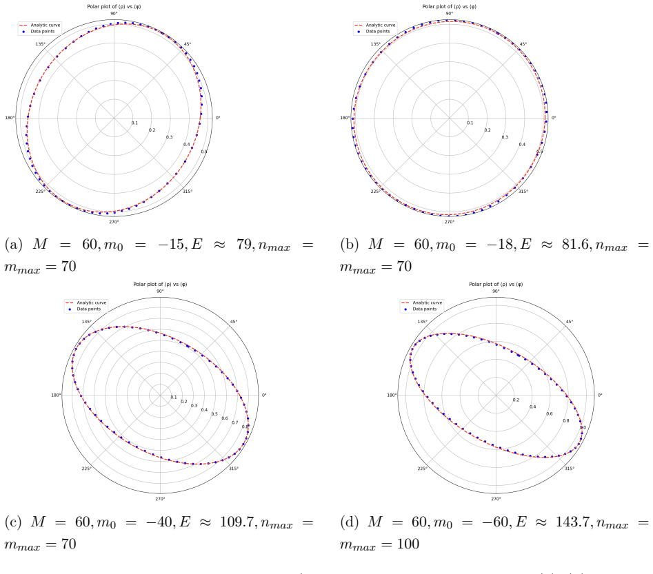
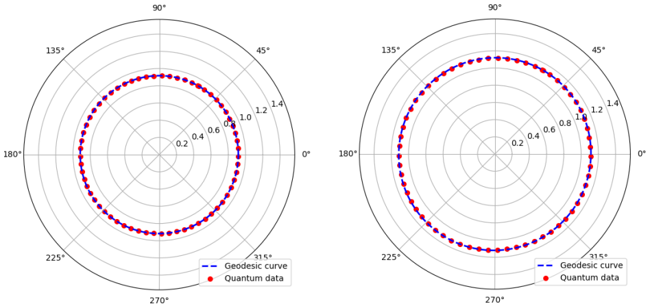
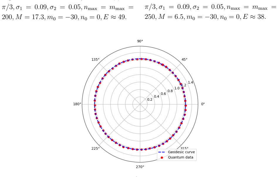
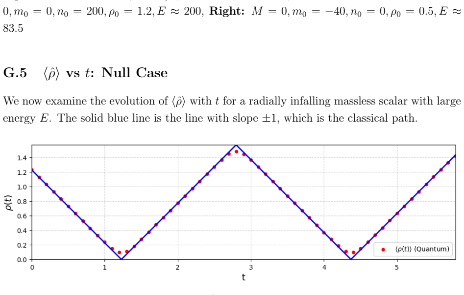
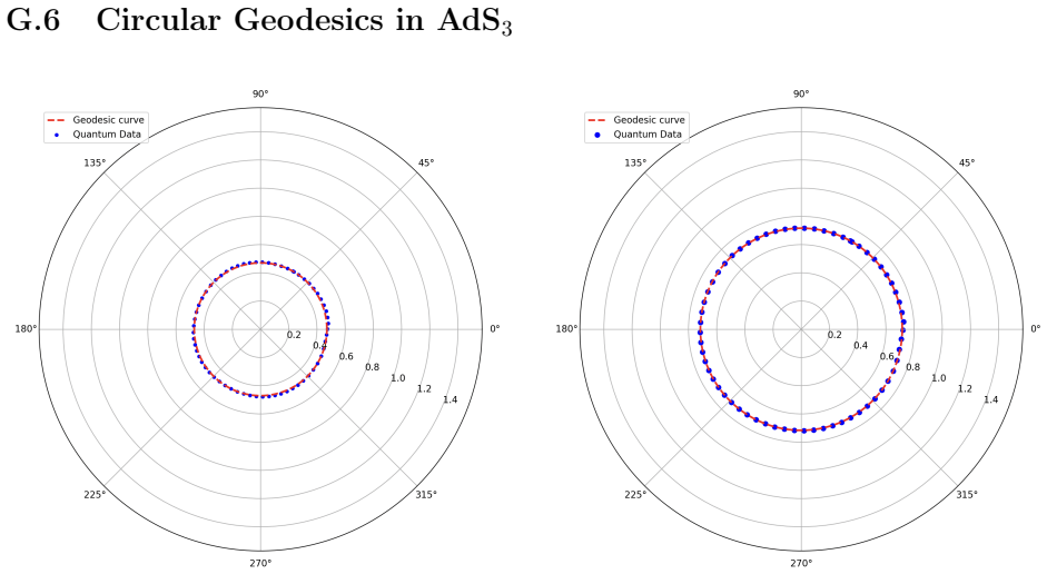
We define a covariant center-of-mass trajectory from the expectation value of the stress tensor operator and show, using only ∇_μ ⟨T^{μν}⟩=0, that it obeys the geodesic equation in the monopole approximation in a general spacetime. We construct position operators from the Klein-Gordon inner product and compute their expectation values in generic single-particle wave packet states, then demonstrate analytically and numerically that both prescriptions reproduce the expected radial, circular, and elliptical-like timelike and null geodesics in empty AdS3, including a controlled ultra-relativistic crossover from timelike to null behavior.
What carries the argument
The covariant center-of-mass trajectory derived from the expectation value of the stress tensor operator, which satisfies the geodesic equation via conservation in the sufficiently localized limit.
If this is right
- This construction supplies a QFT-in-curved-spacetime generalization of the Mathisson-Papapetrou-Dixon framework.
- Explicit wave packets in global AdS3 confirm that both the stress-tensor and position-operator prescriptions reproduce the expected geodesics.
- The wave-packet trajectories exhibit a controlled crossover from timelike to null geodesic behavior in an ultra-relativistic regime.
- Bulk radial localization data is captured by the state's distribution over global descendants of the dual primary on the CFT side.
Where Pith is reading between the lines
- The method could be applied to other backgrounds beyond AdS to extract effective classical trajectories from quantum states.
- It indicates that the semiclassical limit recovers geodesic motion in general relativity from stress-tensor conservation with minimal additional input.
- In holographic settings this supplies a direct link between the organization of CFT states and bulk geodesic motion.
Load-bearing premise
The wave packets must remain localized enough that the monopole approximation holds and the center-of-mass trajectory interpretation does not break down.
What would settle it
An explicit calculation of the center-of-mass trajectory from the stress tensor expectation value for a localized wave packet in AdS3 that deviates from the known geodesic path would falsify the claim.
Figures


read the original abstract
Localized one-particle states of a quantum field theory--whether in flat space or on a curved background--are expected to exhibit geodesic motion in an appropriate semiclassical regime. This expectation is often invoked heuristically: in this work we develop two precise implementations and test them in detail in global AdS$_3$. First, we define a covariant ''center-of-mass'' trajectory from the expectation value of the stress tensor operator and show, using only $\nabla_\mu\langle T^{\mu\nu}\rangle=0$, that it obeys the geodesic equation in the monopole (sufficiently localized) approximation in a general spacetime. This provides a QFT-in-curved-spacetime generalization of the Mathisson-Papapetrou-Dixon framework in classical general relativity. Second, we construct position operators from the Klein--Gordon inner product and mode completeness, and compute their expectation values in generic single-particle wave packet states. We then build explicit normalizable wave packets of a free scalar field in empty AdS$_3$ with tunable energy and angular momentum, and demonstrate analytically and numerically that both prescriptions reproduce the expected radial, circular, and elliptical-like timelike and null geodesics. Our discussion also isolates a natural ultra-relativistic regime in which the wave packet trajectory exhibits a controlled crossover from timelike to null geodesic behavior. We identify precise limits where the localized geodesic interpretation of the wave packet breaks down. On the CFT side, we show that bulk localization--specifically the radial data--is captured by how the state is distributed over global descendants of the dual primary.
Editorial analysis
A structured set of objections, weighed in public.
Referee Report
Summary. The paper defines a covariant center-of-mass worldline from the first moment of the expectation value of the stress-energy tensor in a general curved spacetime and shows, using only the covariant conservation law ∇_μ ⟨T^{μν}⟩ = 0, that this trajectory obeys the geodesic equation under the monopole (sufficiently localized) approximation. It further constructs position operators from the Klein-Gordon inner product and mode completeness, then builds explicit normalizable single-particle wave packets for a free scalar in global AdS₃ with tunable energy and angular momentum. Analytical and numerical results demonstrate that both the stress-tensor and position-operator prescriptions reproduce the expected radial, circular, and elliptical-like timelike and null geodesics, including a controlled ultra-relativistic crossover from timelike to null behavior, while also identifying precise limits where localization fails. The work closes with a CFT-side discussion relating bulk radial localization to the distribution over global descendants of the dual primary.
Significance. If the central derivations hold, the manuscript supplies a parameter-free, first-principles QFT-in-curved-spacetime generalization of the Mathisson-Papapetrou-Dixon framework that recovers geodesic motion directly from stress-tensor conservation. The explicit, normalizable wave-packet constructions in AdS₃, together with both analytic limits and numerical tracking of geodesics, furnish concrete, falsifiable benchmarks for semiclassical regimes and holographic interpretations. The identification of controlled breakdown conditions and the ultra-relativistic crossover further strengthens the result's utility for understanding when the geodesic picture remains valid.
minor comments (2)
- The numerical demonstrations of wave-packet trajectories would benefit from an explicit statement of the discretization scheme, convergence criteria, and quantitative error measures used to establish agreement with the analytic geodesics.
- A short paragraph clarifying the precise sense in which the monopole truncation error is controlled for the AdS₃ wave packets (e.g., via moments of the stress-tensor support) would make the transition from the general-spacetime derivation to the concrete examples more transparent.
Simulated Author's Rebuttal
We thank the referee for their detailed and positive summary of the manuscript, as well as for the recommendation of minor revision. We appreciate the recognition of the central results on the stress-tensor center-of-mass trajectory and the position-operator construction in AdS3.
Circularity Check
No circularity: derivations follow directly from conservation laws and standard QFT constructions
full rationale
The paper's central claim defines the center-of-mass worldline from the first moment of ⟨T^{μν}⟩ and derives the geodesic equation solely from its covariant conservation ∇_μ⟨T^{μν}⟩=0 under the monopole truncation; this is a direct algebraic consequence of the given definition and the Bianchi identity for the stress tensor, with no fitted parameters or self-referential inputs. The second construction uses the standard Klein-Gordon inner product and mode completeness to define position operators whose expectation values are then computed in explicit normalizable wave packets whose dynamics are compared against independently solved geodesic equations in AdS₃. No self-citation chains, ansätze, or uniqueness theorems imported from prior author work appear in the load-bearing steps; the CFT-side statement on global descendants is a direct consequence of the bulk mode expansion rather than a renaming or circular reduction. The derivation chain is therefore self-contained against external benchmarks.
Axiom & Free-Parameter Ledger
axioms (2)
- standard math Conservation of the stress-energy tensor: ∇_μ T^{μν} = 0
- domain assumption Klein-Gordon equation and mode completeness for the scalar field
Lean theorems connected to this paper
-
IndisputableMonolith/Foundation/AlexanderDuality.leanalexander_duality_circle_linking echoes?
echoesECHOES: this paper passage has the same mathematical shape or conceptual pattern as the Recognition theorem, but is not a direct formal dependency.
exact relations d²u/dt² + 4u = … and d²Z/dt² = −Z with u=cos(2ρ), Z=sinρ e^{iϕ}
What do these tags mean?
- matches
- The paper's claim is directly supported by a theorem in the formal canon.
- supports
- The theorem supports part of the paper's argument, but the paper may add assumptions or extra steps.
- extends
- The paper goes beyond the formal theorem; the theorem is a base layer rather than the whole result.
- uses
- The paper appears to rely on the theorem as machinery.
- contradicts
- The paper's claim conflicts with a theorem or certificate in the canon.
- unclear
- Pith found a possible connection, but the passage is too broad, indirect, or ambiguous to say the theorem truly supports the claim.
Reference graph
Works this paper leans on
-
[1]
D. Berenstein and J. Simon,Localized states in global AdS, Phys. Rev. D101(2020) 046026 [arXiv:1910.10227]
-
[2]
CFT descriptions of bulk local states in the AdS black holes
K. Goto and T. Takayanagi,CFT descriptions of bulk local states in the AdS black holes, JHEP10(2017) 153 [arXiv:1704.00053]. 99
work page Pith review arXiv 2017
-
[3]
Terashima, Wave packets in AdS/CFT cor- respondence, Phys
S. Terashima,Wave Packets in AdS/CFT Correspondence, Phys. Rev. D109(2024) 106012, arXiv:2304.08478 [hep-th]
-
[4]
T.D. Newton and E.P. Wigner,Localized States for Elementary Systems, Rev. Mod. Phys.21(1949) 400
work page 1949
-
[5]
A.S.Wightman,On the Localizability of Quantum Mechanical Systems, Rev.Mod.Phys. 34(1962) 845
work page 1962
-
[6]
Hegerfeldt,Remark on causality and particle localization, Phys
G.C. Hegerfeldt,Remark on causality and particle localization, Phys. Rev. D10(1974) 3320
work page 1974
-
[7]
Hegerfeldt,Instantaneous spreading and Einstein causality in quantum theory, Ann
G.C. Hegerfeldt,Instantaneous spreading and Einstein causality in quantum theory, Ann. Phys. (Leipzig)7(1998) 716
work page 1998
-
[8]
A smooth horizon without a smooth horizon,
V. Burman, S. Das and C. Krishnan,A smooth horizon without a smooth horizon, JHEP 2024(2024) 014, doi:10.1007/JHEP03(2024)014 [arXiv:2312.14108 [hep-th]]
-
[9]
A Bottom-Up Approach to Black Hole Microstates,
V. Burman and C. Krishnan,A Bottom-Up Approach to Black Hole Microstates, [arXiv:2409.05850 [hep-th]]
-
[10]
Mathisson,Neue Mechanik materieller Systeme,Acta Phys
M. Mathisson,Neue Mechanik materieller Systeme,Acta Phys. Polon.6(1937) 163
work page 1937
-
[11]
Papapetrou,Spinning test-particles in general relativity
A. Papapetrou,Spinning test-particles in general relativity. I, Proc. Roy. Soc. Lond. A 209(1951) 248
work page 1951
-
[12]
W. G. Dixon,Dynamics of extended bodies in general relativity. I. Momentum and angular momentum,Proc. Roy. Soc. Lond. A314(1970) 499
work page 1970
-
[13]
W. G. Dixon,Dynamics of extended bodies in general relativity. II. Moments of the charge-current vector,Proc. Roy. Soc. Lond. A319(1970) 509
work page 1970
-
[14]
W.G.Dixon,Dynamics of extended bodies in general relativity. III. Equations of motion, Phil. Trans. Roy. Soc. Lond. A277(1974) 59
work page 1974
-
[15]
S.M. Carroll,Spacetime and Geometry: An Introduction to General Relativity, Cam- bridge University Press (2019)
work page 2019
-
[16]
Fleming,Covariant Position Operators, Spin, and Locality, Phys
G.N. Fleming,Covariant Position Operators, Spin, and Locality, Phys. Rev.137(1965) B188
work page 1965
-
[17]
Fleming,Nonlocal Properties of Stable Particles, Phys
G.N. Fleming,Nonlocal Properties of Stable Particles, Phys. Rev.139(1965) B963
work page 1965
-
[18]
Steinmann,Particle Localization in Field Theory, Commun
O. Steinmann,Particle Localization in Field Theory, Commun. Math. Phys.7(1968) 112. 100
work page 1968
-
[19]
Schweber,An Introduction to Relativistic Quantum Field Theory, New York (1961)
S.S. Schweber,An Introduction to Relativistic Quantum Field Theory, New York (1961)
work page 1961
-
[20]
Kalnay,The Localization Problem, inProblems in the Foundations of Physics, M
A.J. Kalnay,The Localization Problem, inProblems in the Foundations of Physics, M. Bunge ed., Springer, New York (1971), pg. 93
work page 1971
-
[21]
Pavšič,Localized states in quantum field theory, [arXiv:1705.02774]
M. Pavšič,Localized states in quantum field theory, [arXiv:1705.02774]
-
[22]
B. Gerlach, D. Gromes, J. Petzold and P. Rosenthal,Über kausales Verhalten nicht- lokaler Größen und Teilchenstruktur in der Feldtheorie, Z. Phys.208(1968) 381
work page 1968
-
[23]
B. Gerlach, D. Gromes and J. Petzold,Energie und Kausalität, Z. Phys.221(1969) 141
work page 1969
-
[24]
Gromes,On the problem of macrocausality in field theory, Z
D. Gromes,On the problem of macrocausality in field theory, Z. Phys.236(1970) 276
work page 1970
-
[25]
S. Weinberg,Gravitation and Cosmology: Principles and Applications of the General Theory of Relativity, John Wiley & Sons, New York (1972)
work page 1972
-
[26]
O. Evnin and C. Krishnan,A Hidden Symmetry of AdS Resonances, Phys. Rev. D91, no.12, 126010 (2015) doi:10.1103/PhysRevD.91.126010 [arXiv:1502.03749 [hep-th]]
-
[27]
J. Kaplan,Lectures on AdS/CFT from the Bottom Up, Department of Physics and Astronomy, Johns Hopkins University
-
[28]
Năstase,Introduction to the AdS/CFT Correspondence, Cambridge University Press, Cambridge (2015)
H. Năstase,Introduction to the AdS/CFT Correspondence, Cambridge University Press, Cambridge (2015)
work page 2015
-
[29]
G. B. Arfken, H. J. Weber, and F. E. Harris,Mathematical Methods for Physicists: A Comprehensive Guide, 7th ed., Academic Press, 2012. 101
work page 2012
discussion (0)
Sign in with ORCID, Apple, or X to comment. Anyone can read and Pith papers without signing in.