Recognition: unknown
Asymptotic Theorems and Averaging in Scalar Field Cosmology
Pith reviewed 2026-05-10 15:06 UTC · model grok-4.3
The pith
Averaging reductions for oscillatory scalar fields yield effective slow dynamics with O(H) error and exact quadrature solutions in cosmology.
A machine-rendered reading of the paper's core claim, the machinery that carries it, and where it could break.
Core claim
For oscillatory scalar fields we derive an averaging reduction to an effective slow system controlled by time averages of dissipation. Uniform derivative bounds together with Barbalat-LaSalle arguments and finite-dimensional center-stable manifold reduction permit late-time analysis. Persistence of equilibria, decay estimates, and local invariant manifolds hold under small C^k perturbations of χ(φ) and G(a). Averaged dissipation lifts to the full oscillatory dynamics with an O(H) error. Exact quadrature solutions in general relativistic, anisotropic, and brane-world cosmologies produce closed-form expressions for t(a), φ(a), and H(a).
What carries the argument
Averaging reduction to an effective slow system, integrated with center-stable manifold reduction and Barbalat-LaSalle invariance principles for late-time analysis.
If this is right
- Equilibria persist and decay estimates hold for the full system when χ(φ) and G(a) receive small C^k perturbations.
- The O(H) error bound quantifies how closely the averaged dissipation approximates the oscillatory dynamics.
- Closed-form t(a), φ(a), and H(a) permit direct analytic evaluation of inflationary observables.
- The reductions and solutions apply directly to anisotropic and brane-world cosmological models.
Where Pith is reading between the lines
- The method could reduce computational cost in early-universe simulations by replacing rapid oscillations with their averaged slow evolution.
- Similar averaging reductions may extend to oscillating fields in other modified-gravity scenarios.
- Confirmation that common potentials satisfy the derivative bounds would broaden applicability to realistic inflationary models.
- The quadrature solutions allow direct analytic comparison of observables across different cosmological frameworks without numerical integration.
Load-bearing premise
Uniform bounds on the derivatives of the oscillatory scalar field are required to justify the averaging reduction and to apply invariance arguments at late times.
What would settle it
A calculation or simulation for a standard potential (quadratic or quartic) in which the scalar field oscillations violate the uniform derivative bounds, causing the late-time decay predictions of the averaged system to deviate from the full dynamics beyond O(H).
Figures


read the original abstract
We present a hybrid study that combines a concise review of scalar-field cosmology with new analytic developments that integrate averaging reductions for oscillatory regimes with dynamical-systems techniques. For oscillatory fields, we derive an averaging reduction that yields an effective slow system whose time averages control dissipation; introducing uniform derivative bounds, Barbalat/LaSalle arguments, and a finite-dimensional center/stable manifold reduction, we carry out late-time analysis of the models. We prove persistence of equilibria, decay estimates, and local invariant manifolds under small $C^k$ perturbations of $\chi(\phi)$ and $G(a)$, quantify how averaged dissipation lifts to the full oscillatory dynamics with an $\mathcal{O}(H)$ error, and provide numerical examples. In addition to asymptotic reductions, we obtain exact quadrature solutions in general relativistic, anisotropic, and brane-world settings, yielding closed-form expressions for $t(a)$, $\phi(a)$, and $H(a)$ and enabling analytic computation of inflationary observables.
Editorial analysis
A structured set of objections, weighed in public.
Referee Report
Summary. The manuscript presents a hybrid analysis of scalar-field cosmology that combines a review of standard models with new analytic results. For oscillatory regimes it derives an averaging reduction to an effective slow system whose dissipation is controlled by time averages; under the additional hypothesis of uniform derivative bounds on the scalar field, it applies Barbalat/LaSalle invariance and center/stable-manifold reduction to obtain late-time asymptotics. The central theorems assert persistence of equilibria, decay estimates, and local invariant manifolds under small C^k perturbations of χ(φ) and G(a), together with an O(H) error bound between the averaged and full dynamics. Independent of the averaging step, the paper also supplies exact quadrature solutions in general-relativistic, anisotropic, and brane-world settings that yield closed-form expressions for t(a), φ(a), and H(a).
Significance. If the uniform derivative bounds can be verified or derived from the Klein-Gordon and Friedmann equations for the potentials under consideration, the persistence and error-estimate results would furnish useful asymptotic control on late-time oscillatory behavior. The exact quadrature solutions constitute a clear, self-contained strength: they furnish closed-form expressions without additional hypotheses and enable direct analytic computation of inflationary observables. The overall significance is therefore conditional on the scope of the derivative-bound assumption.
major comments (1)
- The uniform derivative bounds on the oscillatory scalar field are introduced as an additional hypothesis to justify the averaging reduction and to invoke Barbalat/LaSalle arguments for the late-time analysis. These bounds are not shown to follow from the equations of motion for arbitrary potentials (or even for the standard classes treated in the quadrature section). Because the persistence theorems, decay estimates, local manifold results, and the O(H) lifting of averaged dissipation all rest on this hypothesis, its justification or the precise class of potentials for which it holds is load-bearing for the hybrid asymptotic claims advertised in the title.
Simulated Author's Rebuttal
We thank the referee for the careful reading of the manuscript and for identifying the central role of the uniform derivative bounds in the asymptotic analysis. We address the major comment point by point below and will incorporate clarifications to strengthen the presentation.
read point-by-point responses
-
Referee: The uniform derivative bounds on the oscillatory scalar field are introduced as an additional hypothesis to justify the averaging reduction and to invoke Barbalat/LaSalle arguments for the late-time analysis. These bounds are not shown to follow from the equations of motion for arbitrary potentials (or even for the standard classes treated in the quadrature section). Because the persistence theorems, decay estimates, local manifold results, and the O(H) lifting of averaged dissipation all rest on this hypothesis, its justification or the precise class of potentials for which it holds is load-bearing for the hybrid asymptotic claims advertised in the title.
Authors: We agree that the uniform derivative bounds are introduced as an additional hypothesis and are not derived from the Klein-Gordon and Friedmann equations for arbitrary potentials; the equations alone do not guarantee such bounds in general, as certain potentials can permit growing or irregular oscillations. The asymptotic theorems are therefore scoped to the subclass of potentials for which the oscillatory regime satisfies the stated bounds. For the exact quadrature solutions, the closed-form expressions for t(a), φ(a), and H(a) in the general-relativistic, anisotropic, and brane-world cases permit direct verification that the derivatives remain uniformly bounded for the standard smooth potentials treated (e.g., quadratic potentials yielding explicit periodic-like behavior in the scale factor). We will revise the manuscript by adding a new remark (or short subsection) that explicitly defines the class of potentials to which the averaging reduction and Barbalat/LaSalle arguments apply—namely, those for which sup |dφ/dt| and sup |d²φ/dt²| remain finite over the relevant time intervals, consistent with bounded energy density and regular potential growth. This will also include a brief verification for the quadrature examples and a statement that the exact quadrature results stand independently of the hypothesis. The O(H) error bound and persistence results will be restated with this scope made explicit. revision: yes
Circularity Check
No significant circularity; derivations use explicit assumptions and standard external techniques
full rationale
The paper introduces uniform derivative bounds explicitly as a hypothesis to justify averaging and apply Barbalat/LaSalle arguments, rather than deriving them from its own equations in a self-referential loop. Persistence theorems, decay estimates, and O(H) error quantification rely on center/stable manifold reduction and standard lemmas, which are independent of the paper's fitted quantities or self-citations. Exact quadrature solutions for t(a), φ(a), H(a) are logically separate and do not reduce to the averaging step. No load-bearing step matches self-definitional, fitted-input-called-prediction, or self-citation patterns; the derivation chain remains self-contained against external mathematical benchmarks.
Axiom & Free-Parameter Ledger
axioms (2)
- domain assumption Uniform derivative bounds hold for the oscillatory scalar field
- domain assumption Perturbations of χ(φ) and G(a) are small in the C^k topology
Reference graph
Works this paper leans on
-
[1]
Integrability and Barbalat. If the averaged dissipation f(t) is integrable (as shown for the averaged system), then f(t) = f(t) +O(H(t)),(136) sofremains integrable becauseH∈L 1 loc in the regimes considered and theO(H) term is negligible for large times. Uniform derivative bounds persist under the small additive error, hence Barbalat’s lemma applies to t...
-
[2]
Averaging shows that the averaged invariant region ¯Ψ+ and the true forward invariant set Ψ+ differ by anO(H) tubular neighbourhood for sufficiently smallH
LaSalle invariance and compactness. Averaging shows that the averaged invariant region ¯Ψ+ and the true forward invariant set Ψ+ differ by anO(H) tubular neighbourhood for sufficiently smallH. Since theω-limit of the averaged flow lies at the averaged equilibriumx ∗, the error bound implies theω-limit of the full flow is contained in an arbitrarily small ...
-
[3]
The linearization of the averaged reduced field atx ∗ determines the spectral gap used to obtain exponential convergence onM loc
Spectral gap and manifold persistence. The linearization of the averaged reduced field atx ∗ determines the spectral gap used to obtain exponential convergence onM loc. TheO(H) closeness of the full and averaged vector fields implies the linearizations differ by a small operator perturbation; standard perturbation theory yields continuous dependence of ei...
-
[4]
This requires identifying the critical points and analyzing the eigenvalues of the Jacobian matrix of the linearized flow around each of them
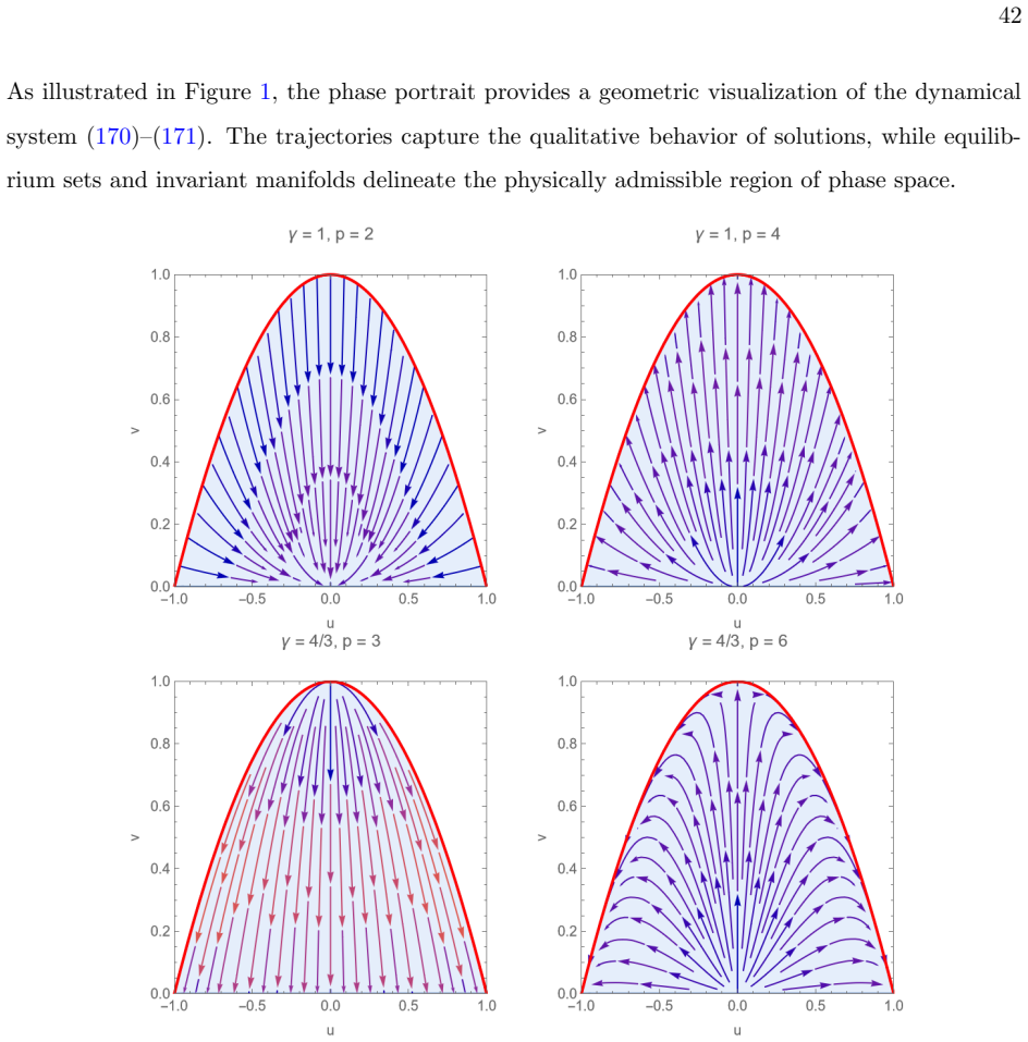
Equilibrium points and stability To understand the local phase-space structure of the system (151), we perform a stability analysis within the framework of qualitative dynamical systems theory. This requires identifying the critical points and analyzing the eigenvalues of the Jacobian matrix of the linearized flow around each of them. Letu= Ω andv= Ωm. Th...
-
[5]
Special parameter cases. In addition to the four isolated equilibria obtained for generic values ofp̸= 3,p̸= 3γ, and γ̸= 1, the system (151) develops continuous families of equilibrium points when the parameters take special values: (i) Casep= 3.Forv= 0 one has A(u,0) =−(p−3)u 2 + (p−3),(166) so whenp= 3 the conditionA(u,0) = 0 holds for allu. Sincev ′ =v...
-
[6]
Dynamical equations inτ-time The dynamical equations inτ-time are the following •Klein–Gordon equation ϕ′′(τ) +a 6(τ) dV dϕ = 0.(196) •Matter continuity equation ρ′ m(τ) + 3γ a′(τ) a(τ) ρm(τ) = 0 =⇒ρ m(τ) =ρ m,0 a(τ) a0 −3γ .(197) •Friedmann equation 3H2(τ) = 1 2a6(τ) ϕ′(τ) 2 +V(ϕ(τ)) +ρ m,0 a(τ) a0 −3γ +G(a(τ)).(198) •Raychaudhuri equation H ′(τ) =− 1 2 ...
-
[7]
(200), (205a) and (205b), allows to obtain a solutiona(t), ϕ(t) for a potentialV(ϕ),the functionsF(a), χ(a), the parametersρ m,0, γ, k, σ0,and Λ, and the integration constantC
Scalar field parametrization and quadrature formalism Defining the potential via V[ϕ(a)] = F(a) a6 ,(200) we obtain the scalar field energy E(τ) = 1 a6(τ) 1 2 ϕ′(τ) 2 +F(a(τ)) .(201) 50 Integrating in standard GR, this energy splits into 1 2 ˙ϕ2 +V(ϕ) = C a6 + 6 a6 Z F(a) a da.(202) The effective Friedmann function becomes: 3H2 ≡ G(a) =G(a) + ρm,0 a3γ + Λ...
-
[8]
Inflationary Parameters in Minimal Coupling FLRW Let us discuss the slow-roll approximation. Two parameters quantify the length of the accel- erated expansion and the smallness of the inflaton’s kinetic energy relative to its potential, which dominates the scalar field energy in slow-roll inflation. For this purpose, the slow-roll parameters are introduce...
-
[9]
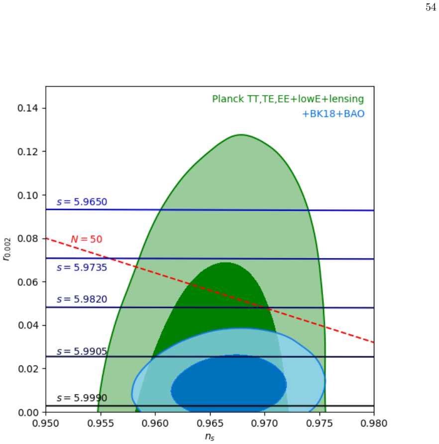
4, we present differentn r-rrelations for a range of values of the parameterswith parameters B,Cfixed to beB= 1 andC= 1
Slow-roll parameters Assuming a potentialV(a) =Ba s−6, we write ϵH(a) = Bas(6−s) +Cs 6Bas +Cs , η H(a) = Bas(s−6) 2 + 6Cs 2Bas(s−6)−2Cs .(220) Alternatively, written in terms of the scalar field potential ϵV (a) = (s−6) 2a−3γ a3γ − 6Bas +s a6G(a) +a 6Λ +C −a 6ρm,0s 12 (B(s−6)a s −Cs) ,(221a) ηV (a) = a−3γ 12(Bas(s−6)−Cs) 2 ρ0,msa6(−Bas(s−6)(s−3(γ+ 2)) +Cs...
2021
-
[10]
Explicit dynamical quantities for scalar source model Assume late-time regime dominated byG(a)≈G(a) + Λ + 6B s as−6. Then, G(a)∼ G∗as−6, G ∗ = 6B s ,ifs >6 Λ,ifs <6 =⇒t(a)≈ R √ 3da a √ G∗as−6 = √ 3√G∗ R a−1−(s−6)/2da= √ 3√G∗ · a(6−s)/2 (6−s)/2 ,ifs >6 q 3 Λ lna,ifs <6 .(226) From above a(t)∼ |6−s| 2 q G∗ 3 t 2/(6−s) ,ifs >6 exp q...
-
[11]
√ B|6−s|√ 2s (t−t 0) # 2 6−s ,(235a) ϕ=ϕ 0 + ln
Scalar field parametrization and quadrature formalism in the early-time limit The early-time limit will be dominated by the termG(a)≈βa −p, whereβrepresents some constant, andp= max{3γ,6,6−s}. Then, one gets t(a)≈ 2 √ 3ap/2 √βp =⇒a(t)≈12 −1/p p βp 2/p t2/p.(231) 56 The scalar field is ϕ(a)≈ 12a p 2 −3 √cs3/2 2F1 1 2 , p−6 2s ; p−6 2s +1; asB(s−6...
-
[12]
•Scalar field evolves asϕ(a)∼ √ 6 lna+ϕ 0 +O(1), implyinga∼e ϕ/ √ 6 asϕ→ −∞
Asymptotic analysis of flat FLRW models Early-time limit (a→0).At early times, the behavior is characterized by •V(ϕ)→ ∞fors <6;V(ϕ)→Bfors= 6. •Scalar field evolves asϕ(a)∼ √ 6 lna+ϕ 0 +O(1), implyinga∼e ϕ/ √ 6 asϕ→ −∞. •The hypergeometric function tends to unity as its argument approaches zero, so the time evolution simplifies to t(a)∼ a3 √ 3C +t 0 +O(a ...
-
[13]
•V(ϕ)→ ∞fors <6;V(ϕ)→Bfors= 6
Case 1: vanishing background terms (ρ m,0 = Λ =C= 0) Early-time limit (a→0). •V(ϕ)→ ∞fors <6;V(ϕ)→Bfors= 6. 60 •ϕ(a)∼const. •t(a)∼ a3 √ 3sσ2 0 +t 0, soa(t)∼(t−t 0)1/3. Late-time limit (a→ ∞). •V(ϕ)→0 fors <6;V(ϕ)→Bfors= 6. •ϕ(a)∼ √6−slna+ϕ 0, soa∼e (ϕ−ϕ0)/√6−s. •t(a)∼σ 1 2 + 3 s 0 a3− s 2 , hencea(t)∼t 1/(3− s 2 )
-
[14]
•a(t)→ ∞, with exponential growtha(t)∼e √ Λ/3t
Case 2: nonzero cosmological constant (Λ>0, s= 3) Late-time limit (t→ ∞). •a(t)→ ∞, with exponential growtha(t)∼e √ Λ/3t . •H(t)→ p Λ/3. •q(t)→ −1, confirming accelerated expansion. •V(ϕ)→0, consistent with scalar field dilution. Early-time limit (t→t 0). •In generala(t)→0, withV(ϕ)→const ift 0 = ln(B− √ Λσ0)√ 3Λ . •ϕ(t)→ ∞ift 0 = ln(B− √ Λσ0)√ 3Λ . •Dyna...
-
[15]
Inflationary parameters in Bianchi I cosmology We analyze the slow-roll parameters for the Bianchi I solution with scalar sourceF(a) =Ba s, assuming minimal coupling and vanishing background terms ρm,0 = Λ =C= 0.(249) The scalar field kinetic term is given by L(a) = 6−s s Bas−6,(250) and the Friedmann function includes anisotropic shear: G(a) = 6B sa6−s +...
-
[16]
Slow-roll parameters in flat FLRW cosmology with interaction Assumingk= Λ =C= 0, we consider the interacting scalar field model in a flat FLRW background. The slow-roll parameters are defined as ϵH(a) = 1 + F(a) ρm,0a6−3γχ(a) 3γ 2 −2 −3 R 2F(a) a −(γ−2)ρ m,0a5−3γχ(a) 3γ 2 −2 da ,(268a) ηH(a) = aF ′(a) 2 h ρm,0a6−3γχ(a) 3γ 2 −2 −3 R 2F(a) a −(γ−2)ρ m,0a5−3...
2025
-
[17]
096/2022, and through the N´ ucleo de Investigaci´ on en Simetr´ ıas y la Estructura del Universo (NISEU), Resolution VRIDT No
We also extend our gratitude to the Vicerrector´ ıa de Investigaci´ on y Desarrollo Tecnol´ ogico (VRIDT) of UCN for the scientific support provided through the N´ ucleo de Investigaci´ on en Ge- ometr´ ıa Diferencial y Aplicaciones, Resolution VRIDT No. 096/2022, and through the N´ ucleo de Investigaci´ on en Simetr´ ıas y la Estructura del Universo (NIS...
2022
-
[18]
A. H. Guth, Physical Review D23, 347 (1981)
1981
-
[19]
Jordan,Research on the theory of general relativity(1958), iNSPIRE citation
P. Jordan,Research on the theory of general relativity(1958), iNSPIRE citation
1958
-
[20]
Brans and R
C. Brans and R. H. Dicke, Physical Review124, 925 (1961)
1961
-
[21]
G. W. Horndeski, International Journal of Theoretical Physics10, 363 (1974)
1974
-
[22]
Ibanez, R
J. Ibanez, R. J. van den Hoogen, and A. A. Coley, Physical Review D51, 928 (1995)
1995
-
[23]
A. A. Coley, J. Ibanez, and R. J. van den Hoogen, Journal of Mathematical Physics38, 5256 (1997)
1997
- [24]
-
[25]
A. Coley and M. Goliath, Classical and Quantum Gravity17, 2557 (2000), gr-qc/0003080
-
[26]
A. Coley and M. Goliath, Physical Review D62, 043526 (2000), gr-qc/0004060
-
[27]
Foster, Classical and Quantum Gravity15, 3485 (1998), gr-qc/9806098
S. Foster, Classical and Quantum Gravity15, 3485 (1998), gr-qc/9806098
-
[28]
Miritzis, Classical and Quantum Gravity20, 2981 (2003), gr-qc/0303014
J. Miritzis, Classical and Quantum Gravity20, 2981 (2003), gr-qc/0303014
-
[29]
D. G. Morales and Y. N. Alvarez,Quintaesencia con acoplamiento no m´ ınimo a la materia oscura desde la perspectiva de los sistemas din´ amicos(2008), bachelor Thesis, Universidad Central Marta Abreu de Las Villas
2008
-
[30]
Leon, Classical and Quantum Gravity26, 035008 (2009), 0812.1013
G. Leon, Classical and Quantum Gravity26, 035008 (2009), 0812.1013
-
[31]
R. Giambo and J. Miritzis, Classical and Quantum Gravity27, 095003 (2010), 0908.3452
-
[32]
M. Shahalam, R. Myrzakulov, and M. Y. Khlopov, General Relativity and Gravitation51, 125 (2019), 1905.06856
- [33]
-
[34]
F. Humieja and M. Szyd lowski, European Physical Journal C79, 794 (2019), 1901.06578. 72
- [35]
- [36]
- [37]
- [38]
-
[39]
G. Le´ on Torres, Ph.D. thesis, Marta Abreu Central U., Cuba (2010), 1412.5665
-
[40]
G. Leon and C. R. Fadragas,Cosmological dynamical systems(LAP Lambert Academic Publishing, 2012), ISBN 978-3-8473-0233-9, 1412.5701
- [41]
-
[42]
G. Leon and F. O. F. Silva, Class. Quant. Grav.38, 015004 (2021), 2007.11990
-
[43]
G. Leon and F. O. F. Silva, Class. Quant. Grav.37, 245005 (2020), 2007.11140
-
[44]
G. Leon and F. O. F. Silva,Generalized scalar field cosmologies(2019), 1912.09856
- [45]
-
[46]
G. Leon and C. Michea,Averaging Theory and Dynamical Systems in Cosmology: A Qualitative Study of Oscillatory Scalar-Field Models(2026), 2601.17157
- [47]
-
[48]
A. A. Coley, inSpanish Relativity Meeting (ERE 99)(1999), gr-qc/9910074
work page internal anchor Pith review arXiv 1999
-
[49]
T. Gonzalez and I. Quiros, Class. Quant. Grav.25, 175019 (2008), 0707.2089
- [50]
- [51]
- [52]
-
[53]
Fajman, G
D. Fajman, G. Heißel, and J. W. Jang, Class. Quant. Grav.38, 085005 (2021)
2021
- [54]
- [55]
- [56]
-
[57]
N. Kaloper and K. A. Olive, Phys. Rev. D57, 811 (1998), hep-th/9708008
-
[58]
Carr,Applications of Centre Manifold Theory, vol
J. Carr,Applications of Centre Manifold Theory, vol. 35 ofApplied Mathematical Sciences(Springer- Verlag, New York, 1981), ISBN 0-387-90577-4
1981
-
[59]
Giambo, F
R. Giambo, F. Giannoni, and G. Magli, Classical and Quantum Gravity20, 4943 (2003)
2003
-
[60]
Giambo, F
R. Giambo, F. Giannoni, and G. Magli, Symmetry7, 2303 (2015)
2015
-
[61]
Corona and R
A. Corona and R. Giambo, Symmetry16, 583 (2024)
2024
-
[62]
J. P. LaSalle, Journal of Differential Equations4, 57 (1968). 73
1968
-
[63]
Wiggins,Introduction to Applied Nonlinear Dynamical Systems and Chaos, vol
S. Wiggins,Introduction to Applied Nonlinear Dynamical Systems and Chaos, vol. 2 ofTexts in Applied Mathematics(Springer, 2003), 2nd ed
2003
- [64]
-
[65]
Planck 2018 results. VI. Cosmological parameters
N. Aghanim et al. (Planck), Astron. Astrophys.641, A6 (2020), [Erratum: Astron.Astrophys. 652, C4 (2021)], 1807.06209
work page internal anchor Pith review Pith/arXiv arXiv 2020
-
[66]
P. A. R. Ade et al. (BICEP2, Keck Array), Phys. Rev. Lett.121, 221301 (2018), 1810.05216
work page Pith review arXiv 2018
-
[67]
D. Camarena and V. Marra, Phys. Rev. Research2, 013028 (2020), astro-ph.CO/1906.11814
discussion (0)
Sign in with ORCID, Apple, or X to comment. Anyone can read and Pith papers without signing in.