Recognition: unknown
An improvement of model-independent method for meson charge radius calculation
Pith reviewed 2026-05-10 13:42 UTC · model grok-4.3
The pith
Introducing an auxiliary function of momentum transfer squared further suppresses higher-order terms in model-independent lattice calculations of meson charge radii.
A machine-rendered reading of the paper's core claim, the machinery that carries it, and where it could break.
Core claim
By introducing an auxiliary function of the momentum transfer squared and reformulating the method in terms of its product with the form factor rather than the form factor itself, higher-order contributions are further suppressed, notably in cases of small volume and large radius. Applying this method to mock data based on a monopole form factor as well as to actual lattice QCD data reduces residual finite-volume effects and provides an effective framework for meson charge radius determinations.
What carries the argument
An auxiliary function of the squared momentum transfer (implemented as quadratic or logarithmic) whose product with the form factor is inserted into the spatial-moment formulas, thereby shifting the leading truncation error to higher order.
If this is right
- Residual finite-volume effects in the charge radius are smaller than in the earlier model-independent approach for the same lattice size.
- The method remains free of any assumed functional form for the form factor.
- Quadratic and logarithmic auxiliary functions both work on monopole mock data and on the tested Nf=2+1 ensembles.
- The improvement is largest precisely when the physical radius is large relative to the lattice size.
Where Pith is reading between the lines
- Smaller lattices could become usable for radius determinations, lowering the computational cost of reaching a given precision.
- The same auxiliary-function reformulation might be portable to other lattice quantities extracted from spatial moments, such as higher derivatives or transition form factors.
- If the suppression remains effective across a broader class of form-factor shapes, the technique could become the default model-independent route for electromagnetic radii.
Load-bearing premise
That quadratic and logarithmic auxiliary functions will suppress higher-order contributions for any unknown true shape of the form factor without introducing new biases.
What would settle it
A comparison on a very large-volume ensemble showing whether radii extracted with the new auxiliary-function method agree with those from a high-precision multi-point fit while the older moment method still deviates.
Figures


read the original abstract
We propose a variant of the model-independent method for determining meson charge radii from spatial moments of correlation functions on the lattice. Traditional determinations based on fits to the momentum transfer squared dependence of form factors are subject to systematic uncertainties arising from the choice of fit ansatz. By contrast, model-independent methods based on spatial moments provide a useful framework for determining the slope of the form factor without assuming its functional form. Recently, Feng et al. proposed a model-independent method, which drastically suppresses the finite-volume effect in the charge radius coming from higher-order contributions of the expansion of the form factor with respect to the momentum transfer squared. In this work, we introduce an auxiliary function of the momentum transfer squared and reformulate the method in terms of its product with the form factor, rather than the form factor itself, thereby further suppressing higher-order contributions, notably in cases of small volume and large radius. In particular, we investigate quadratic and logarithmic forms as practical choices for this auxiliary function. Applying this method to mock data based on a monopole form factor, as well as to actual lattice QCD data using $N_f=2+1$ gauge ensembles at $m_\pi \simeq 0.5$ and $0.3$ GeV, we find that it reduces residual finite-volume effects and provides an effective framework for meson charge radius determinations.
Editorial analysis
A structured set of objections, weighed in public.
Referee Report
Summary. The manuscript proposes an improvement to the model-independent method of Feng et al. for extracting meson charge radii from lattice QCD spatial moments of correlation functions. The authors introduce an auxiliary function f(Q²) of the squared momentum transfer (considering quadratic and logarithmic choices) and reformulate the extraction procedure in terms of the product f(Q²) × F(Q²) rather than F(Q²) alone. This is claimed to further suppress higher-order terms in the small-Q² expansion, thereby reducing residual finite-volume effects in the charge radius, particularly for small volumes and large radii. The method is tested on mock data generated from a monopole form factor and applied to two N_f=2+1 gauge ensembles at m_π ≈ 0.5 and 0.3 GeV.
Significance. If the central claim holds, the approach would offer a practical enhancement to existing model-independent techniques for lattice determinations of hadron charge radii, potentially allowing more reliable extractions on smaller volumes without sacrificing the avoidance of fit ansatz biases. The direct mathematical re-expression preserves the model-independent character in principle, which is a methodological strength.
major comments (3)
- [§4.1] §4.1 (mock data tests): The suppression of finite-volume effects and absence of bias from the auxiliary function are demonstrated exclusively on mock data generated assuming a monopole form factor. This does not test whether quadratic or logarithmic choices alter the extracted radius when the true form factor contains different higher-order structure (e.g., dipole or resonance contributions), which is load-bearing for the claim of improved model independence.
- [§3] §3 (reformulation): The derivation of the product f(Q²) × F(Q²) and the corresponding spatial-moment expression does not explicitly quantify how the auxiliary-function coefficients enter the final radius extraction or demonstrate that they remain free of new systematic bias when the true form factor deviates from the test case; this step is central to asserting further suppression without compromising the result.
- [§4.2] §4.2 (lattice ensembles): The application to the two N_f=2+1 ensembles reports reduced residual finite-volume effects but provides no tabulated quantitative comparison (e.g., radius values and uncertainties with/without the auxiliary function, or explicit FV correction magnitudes), leaving the magnitude of the claimed improvement unverifiable.
minor comments (2)
- [§3] The notation for the auxiliary function and its product with the form factor should be introduced with an explicit example expansion up to O(Q⁴) to clarify the suppression mechanism.
- [§4] Figure captions for the mock-data and ensemble results should include the specific auxiliary-function parameters used and the volume sizes to aid reproducibility.
Simulated Author's Rebuttal
We thank the referee for the careful reading of our manuscript and the constructive comments. We address each major point below and indicate the revisions we will make to improve clarity and verifiability.
read point-by-point responses
-
Referee: [§4.1] §4.1 (mock data tests): The suppression of finite-volume effects and absence of bias from the auxiliary function are demonstrated exclusively on mock data generated assuming a monopole form factor. This does not test whether quadratic or logarithmic choices alter the extracted radius when the true form factor contains different higher-order structure (e.g., dipole or resonance contributions), which is load-bearing for the claim of improved model independence.
Authors: The reformulation is derived generally, without assuming any specific form for F(Q²). The auxiliary function f(Q²) is selected to reduce the size of Q⁴ and higher coefficients in the expansion of the product around Q²=0, independent of the coefficients present in F. The charge radius is recovered from the slope of the product after a known correction from f, preserving model independence. To strengthen the demonstration, we will add mock-data tests with dipole and resonance-inspired form factors in the revised §4.1. revision: yes
-
Referee: [§3] §3 (reformulation): The derivation of the product f(Q²) × F(Q²) and the corresponding spatial-moment expression does not explicitly quantify how the auxiliary-function coefficients enter the final radius extraction or demonstrate that they remain free of new systematic bias when the true form factor deviates from the test case; this step is central to asserting further suppression without compromising the result.
Authors: We will expand the derivation in the revised §3 to show the explicit Taylor expansion of the product, demonstrating that the auxiliary coefficients affect only the Q⁴ and higher terms while the linear term (which determines the radius) receives a known, exact adjustment from f. Because the spatial-moment relation is applied to the product and the procedure remains exact in infinite volume, no new systematic bias is introduced when F deviates from the monopole case. revision: partial
-
Referee: [§4.2] §4.2 (lattice ensembles): The application to the two N_f=2+1 ensembles reports reduced residual finite-volume effects but provides no tabulated quantitative comparison (e.g., radius values and uncertainties with/without the auxiliary function, or explicit FV correction magnitudes), leaving the magnitude of the claimed improvement unverifiable.
Authors: We agree that tabulated comparisons are required for verifiability. In the revised §4.2 we will insert a table listing the extracted radii (with uncertainties) obtained both with and without the auxiliary function for each ensemble, together with the estimated residual finite-volume corrections. This will make the size of the improvement quantitative and directly comparable. revision: yes
Circularity Check
No circularity: reformulation is an independent mathematical re-expression with external validation.
full rationale
The paper's central step is a direct algebraic reformulation of the Feng et al. spatial-moment method by multiplying the form factor by a chosen auxiliary function of Q^2 (quadratic or logarithmic) to suppress higher-order terms in the small-volume expansion. This re-expression does not define the radius in terms of itself, nor rename a fitted parameter as a prediction, nor invoke any self-citation chain for uniqueness or ansatz justification. The auxiliary forms are presented as practical choices and are validated on independent monopole mock data plus two external Nf=2+1 ensembles; the derivation chain therefore remains self-contained against external benchmarks and does not reduce to its inputs by construction.
Axiom & Free-Parameter Ledger
free parameters (1)
- auxiliary function coefficients
axioms (2)
- domain assumption The electromagnetic form factor of the meson admits a Taylor expansion in powers of Q^2 around zero momentum transfer.
- domain assumption Finite-volume corrections to the form factor can be organized as an expansion in momentum transfer whose higher terms are suppressible by weighting with an auxiliary function.
Reference graph
Works this paper leans on
-
[1]
If the parameters satisfy the condition s2 =f 2 +f 1g1 +g 2 = 0,(46) the higher-order contribution completely vanishes
Quadratic function For this mock data expressed by the monopole formF(Q 2), we chooseG(Q 2) to be a quadratic function ofQ 2: G(Q2) = 1 +g 1Q2 +g 2Q4,(45) whereg 1 andg 2 are parameters. If the parameters satisfy the condition s2 =f 2 +f 1g1 +g 2 = 0,(46) the higher-order contribution completely vanishes. The reason is that sn =f 1sn−1 = 0,(47) forn≥3 1, ...
-
[2]
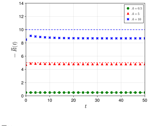
logarithmic function Another example of the choice ofG(Q 2) is a logarithmic function given by G(Q2) = 1 +g l 1 log(1 +g l 2Q2).(53) 15 t 0 10 20 30 40 50 −R( t) 0 2 4 6 8 10 12 14 L= 16 L= 32 L= 64 L= 128 FIG. 8. Results of−R(t) from the mock data using our method with the quadratic function for G(Q2) withg 1 = 0 forL= 16,32,64,and 128 withA= 10 as a fun...
-
[3]
Thus, we choose the same reference time,t r = 25, as in the previous example to examine theg l 1 dependence ofR 2(t)
Although in a smallertregion,R 2(t) slightly depends ont, it is reasonably flat in a large-tregion. Thus, we choose the same reference time,t r = 25, as in the previous example to examine theg l 1 dependence ofR 2(t). The value ofR 2(tr) is plotted in Fig. 10 as a function ofg l 1 in fourg l 2 cases. As in the polynomialG(Q 2) case,R 2(tr) reasonably beha...
1954
-
[4]
In fact, our data show a slight deviation from unity, as seen in Fig
Analysis of Amplitude Ratio Although the ratioR Z(Q2) =Z π(p)/Zπ(0) should be unity in the continuum theory, it is not exactly unity at finite lattice spacing. In fact, our data show a slight deviation from unity, as seen in Fig. 18. Since correctly evaluating the effects originating fromR Z(Q2) is impor- tant for a reliable determination of the charge ra...
-
[5]
linear”, “quad
Analysis of charge radius In our method, we employ a quadratic functionG(Q2) = 1+g 1Q2+g2Q4 and a logarithmic functionG(Q 2) = 1 +g l 1 log(1 +g l 2Q2), as discussed in the previous section. In both cases, the parameter sets are determined fromR 2(t) = 0 defined in Eq. (48). An example of the data forR 2(t) = 0 with the quadratic function is plotted in Fi...
-
[6]
Pohl et al., Nature466, 213 (2010)
R. Pohl et al., Nature466, 213 (2010)
2010
-
[7]
Navas et al
S. Navas et al. (Particle Data Group), Phys. Rev. D110, 030001 (2024)
2024
- [8]
- [9]
-
[10]
J. Koponen, F. Bursa, C. T. H. Davies, R. J. Dowdall, and G. P. Lepage, Phys. Rev. D93, 054503 (2016), arXiv:1511.07382 [hep-lat]
-
[11]
C. Alexandrou et al. (ETM), Phys. Rev. D97, 014508 (2018), arXiv:1710.10401 [hep-lat]
- [12]
- [13]
-
[14]
U. Aglietti, G. Martinelli, and C. T. Sachrajda, Phys. Lett. B324, 85 (1994), arXiv:hep- lat/9401004
-
[15]
L. Lellouch, J. Nieves, C. T. Sachrajda, N. Stella, H. Wittig, G. Martinelli, and D. G. Richards (UKQCD), Nucl. Phys. B444, 401 (1995), arXiv:hep-lat/9410013
-
[16]
C. Alexandrou, A. Athenodorou, M. Constantinou, K. Hadjiyiannakou, K. Jansen, G. Kout- sou, K. Ottnad, and M. Petschlies, Phys. Rev. D93, 074503 (2016), arXiv:1510.05823 [hep- lat]
-
[17]
C. Bouchard, C. C. Chang, K. Orginos, and D. Richards, PoSLATTICE2016, 170 (2016), arXiv:1610.02354 [hep-lat]
-
[18]
C. Alexandrou, M. Constantinou, G. Koutsou, K. Ottnad, and M. Petschlies (ETM), Phys. Rev. D94, 074508 (2016), arXiv:1605.07327 [hep-lat]
- [19]
-
[20]
C. Alexandrou, K. Hadjiyiannakou, G. Koutsou, K. Ottnad, and M. Petschlies, Phys. Rev. D101, 114504 (2020), arXiv:2002.06984 [hep-lat]
-
[21]
K.-I. Ishikawa, Y. Kuramashi, S. Sasaki, E. Shintani, and T. Yamazaki (PACS), Phys. Rev. D104, 074514 (2021), arXiv:2107.07085 [hep-lat]
- [22]
- [23]
- [24]
- [25]
-
[26]
K.-i. Ishikawa, N. Ishizuka, Y. Kuramashi, Y. Namekawa, Y. Taniguchi, N. Ukita, T. Ya- mazaki, and T. Yoshi´ e (PACS), Phys. Rev. D106, 094501 (2022), arXiv:2206.08654 [hep-lat]
-
[27]
T. Yamazaki, K.-i. Ishikawa, Y. Kuramashi, and A. Ukawa, Phys.Rev.D86, 074514 (2012), arXiv:1207.4277 [hep-lat]
-
[28]
J. Kakazu, K.-i. Ishikawa, N. Ishizuka, Y. Kuramashi, Y. Nakamura, Y. Namekawa, Y. Taniguchi, N. Ukita, T. Yamazaki, and T. Yoshi´ e (PACS), Phys. Rev. D101, 094504 (2020), arXiv:1912.13127 [hep-lat]
-
[29]
G. W. Kilcup, S. R. Sharpe, R. Gupta, G. Guralnik, A. Patel, and T. Warnock, Phys. Lett. B164, 347 (1985)
1985
-
[30]
Martinelli and C
G. Martinelli and C. T. Sachrajda, Nucl. Phys. B316, 355 (1989)
1989
- [31]
-
[32]
Kakazu, K.-I
J. Kakazu, K.-I. Ishikawa, N. Ishizuka, Y. Kuramashi, Y. Nakamura, Y. Namekawa, Y. Taniguchi, N. Ukita, T. Yamazaki, and T. Yoshie (PACS), PoSLATTICE2016, 160 (2017)
2017
-
[33]
D. Br¨ ommelet al. (QCDSF/UKQCD), Eur. Phys. J. C51, 335 (2007), arXiv:hep-lat/0608021
- [34]
- [35]
-
[36]
T. Yamazaki, K.-i. Ishikawa, Y. Kuramashi, and A. Ukawa, Phys. Rev.D92, 014501 (2015), arXiv:1502.04182 [hep-lat]. Appendix A: Size of finite-volume effect in model-independent methods In this appendix, the finite-volume effect in model-independent methods is estimated with mock data discussed in Sec. III. In addition to the three methods discussed in the...
-
[37]
linear”, “quad
Modified monopole form factor forL= 32andm π = 0.5GeV Our improved method with the logarithmic function gives a larger⟨r 2⟩onL= 32 at mπ = 0.5 GeV than that onL= 64, as shown in Fig. 23. To understand this systematic error, we employ a modified monopole form forF π(Q2) given by Fπ(Q2) = 1 +CQ 6 1 +AQ 2 ,(A3) where we chooseA= 5.75 andC= 12 to reproduce th...
-
[38]
We set the reference time t= 20, which is a similar value to that in Ref
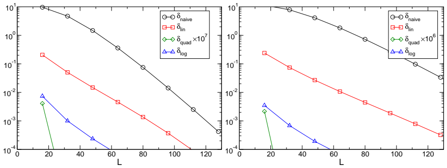
Parameters for the physicalm π The results ofδ J are evaluated using the mock data with the parameters for the physical point,m π = 0.135 GeV and⟨r 2⟩= 0.44 fm 2 ata= 0.08 fm. We set the reference time t= 20, which is a similar value to that in Ref. [30]. In this calculation, the exact monopole form andR Z(Q2) = 1 are adopted. Figure 27 shows thatδ lin is...
2095
discussion (0)
Sign in with ORCID, Apple, or X to comment. Anyone can read and Pith papers without signing in.