Recognition: unknown
A minimal implementation of Yang-Mills theory on a digital quantum computer
Pith reviewed 2026-05-10 09:47 UTC · model grok-4.3
The pith
Simplified Hamiltonians enable a minimal implementation of SU(N) Yang-Mills theory for digital quantum simulation.
A machine-rendered reading of the paper's core claim, the machinery that carries it, and where it could break.
Core claim
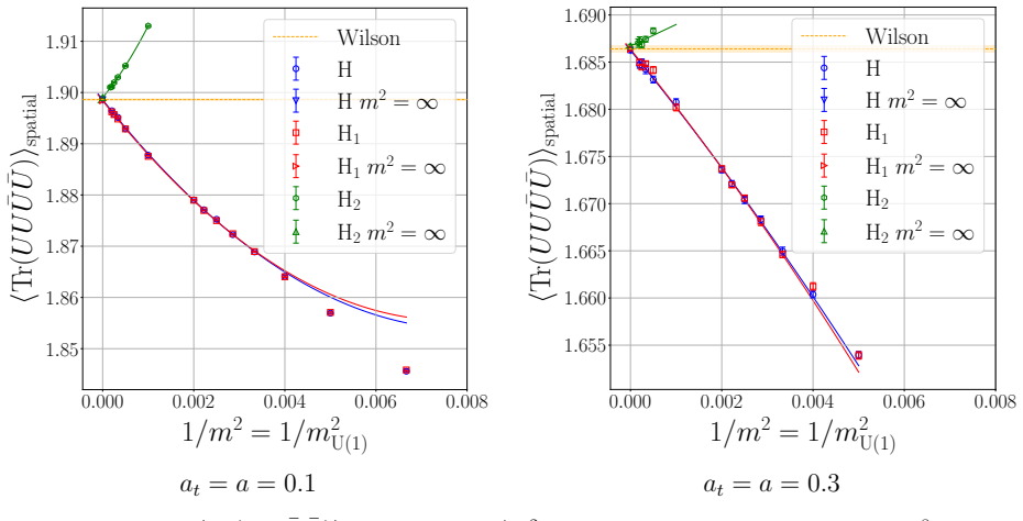
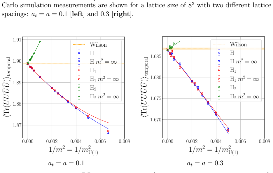
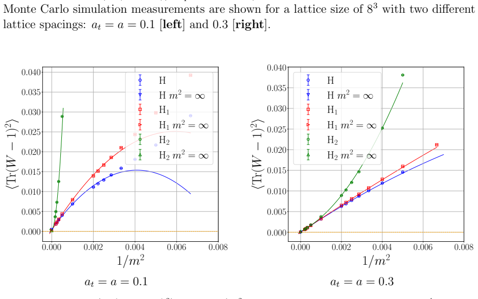
The authors show that simplified Hamiltonians together with improved convergence techniques allow the orbifold lattice formulation to reach the Kogut-Susskind Hamiltonian without a large scalar mass. For SU(2) the isomorphism SU(2) congruent to S^3 embedded in R^4 reduces the local degrees of freedom further. These modifications are validated by Euclidean Monte Carlo benchmarks that confirm the modified theories approach standard Yang-Mills in the appropriate limit.
What carries the argument
The orbifold lattice simulation protocol with logarithmic scaling in local Hilbert-space truncation, combined with simplified Hamiltonians and convergence methods to the infinite-mass limit of the Kogut-Susskind Hamiltonian.
If this is right
- Resource requirements for digital quantum simulation of SU(N) Yang-Mills are reduced beyond the original logarithmic scaling.
- Simulations become viable without auxiliary large scalar masses.
- SU(2) calculations gain an additional reduction via the R^4 embedding of the group manifold.
- Monte Carlo benchmarks establish that the new analytical improvements preserve the target continuum limit.
- The noncompact-variable approach gains concrete support as a route toward quantum simulations of non-Abelian gauge theories.
Where Pith is reading between the lines
- The framework could be tested on present-day quantum hardware for small lattices to measure actual qubit and gate counts.
- Similar Hamiltonian simplifications might apply to other non-Abelian groups or to theories that include dynamical fermions.
- If the error bounds hold, the method opens a path to studying confinement and other strong-coupling phenomena with quantum resources.
- Connections to alternative noncompact lattice formulations could be checked by comparing spectra or correlation functions.
Load-bearing premise
The simplified Hamiltonians and convergence methods accurately reproduce the Kogut-Susskind Hamiltonian in the infinite-mass limit without introducing uncontrolled errors.
What would settle it
A direct quantum simulation or Monte Carlo comparison that produces plaquette expectation values or Wilson-loop observables deviating from the standard Kogut-Susskind theory in the infinite-mass limit would falsify the accuracy claim.
Figures


read the original abstract
We present a minimal implementation of SU($N$) pure Yang-Mills theory in $3+1$ dimensions for digital quantum simulation, designed to enable quantum advantage. Building on the orbifold lattice simulation protocol with logarithmic scaling in the local Hilbert-space truncation, we introduce further simplified Hamiltonians. Furthermore, we test simple methods that improve the convergence to the infinite mass limit, thereby removing the requirement of a large scalar mass to obtain the Kogut-Susskind Hamiltonian. For the SU(2) theory, we can cut the resource requirement further by utilizing the embedding of $\mathrm{SU}(2)\cong\mathrm{S}^3$ into $\mathbb{R}^4$. Monte Carlo simulations of the Euclidean path integral were used to benchmark the accuracy of these new analytical improvements to the theory. These results provide further support for the noncompact-variable-based approach as a practical framework for quantum simulation of non-Abelian gauge theories.
Editorial analysis
A structured set of objections, weighed in public.
Referee Report
Summary. The manuscript presents a minimal implementation of SU(N) pure Yang-Mills theory in 3+1 dimensions designed for digital quantum computers. It extends the orbifold lattice protocol by introducing simplified Hamiltonians and convergence improvement methods to achieve the Kogut-Susskind Hamiltonian in the infinite-mass limit without requiring large scalar masses. For SU(2), it leverages the SU(2) ≅ S^3 embedding in R^4 to further reduce resources. The analytical improvements are benchmarked using Monte Carlo simulations of the Euclidean path integral, which the authors argue provide support for the noncompact-variable approach as a practical quantum simulation framework.
Significance. Should the benchmarks confirm that the simplifications introduce no uncontrolled errors in recovering the standard Kogut-Susskind formulation, this work would represent a meaningful advance in reducing the computational resources needed for quantum simulations of non-Abelian gauge theories. The logarithmic scaling and minimal implementation could help bridge the gap to quantum advantage in this area. The use of independent Monte Carlo benchmarks to validate the approach is a constructive element, though stronger quantitative validation would enhance its significance.
major comments (1)
- [Benchmarking with Monte Carlo simulations] The central support for the claim that the simplified Hamiltonians and convergence methods accurately reproduce the Kogut-Susskind Hamiltonian in the infinite-mass limit comes from Monte Carlo benchmarks of the Euclidean path integral. However, no explicit quantitative error analysis, finite-mass comparison plots against the unmodified KS Hamiltonian, or statements on how truncation or orbifold artifacts are controlled are provided. This leaves the systematic errors unquantified and is load-bearing for the quantum-simulation applicability asserted in the abstract.
minor comments (1)
- [Abstract] The abstract states that 'Monte Carlo simulations ... were used to benchmark the accuracy of these new analytical improvements' but omits any mention of specific error metrics, resource counts, or comparison baselines, which would strengthen the summary of the results.
Simulated Author's Rebuttal
We thank the referee for their careful reading of the manuscript and for the constructive feedback. We agree that additional quantitative details on the Monte Carlo benchmarks would strengthen the support for our claims and will revise the manuscript accordingly.
read point-by-point responses
-
Referee: [Benchmarking with Monte Carlo simulations] The central support for the claim that the simplified Hamiltonians and convergence methods accurately reproduce the Kogut-Susskind Hamiltonian in the infinite-mass limit comes from Monte Carlo benchmarks of the Euclidean path integral. However, no explicit quantitative error analysis, finite-mass comparison plots against the unmodified KS Hamiltonian, or statements on how truncation or orbifold artifacts are controlled are provided. This leaves the systematic errors unquantified and is load-bearing for the quantum-simulation applicability asserted in the abstract.
Authors: We acknowledge the referee's concern. The Monte Carlo results presented in the manuscript already illustrate convergence of the simplified Hamiltonians toward the expected Kogut-Susskind behavior as the scalar mass is increased, with statistical errors shown. However, we agree that the current presentation would benefit from more explicit quantitative error analysis, direct comparison plots at finite mass against the unmodified Kogut-Susskind Hamiltonian, and additional statements clarifying how truncation and orbifold artifacts are controlled. In the revised version we will add these elements, including error bars on the deviation from the target Hamiltonian and a dedicated discussion of artifact suppression. revision: yes
Circularity Check
No significant circularity; central benchmarks use independent Monte Carlo simulations
full rationale
The paper builds on an orbifold lattice protocol and introduces simplified Hamiltonians plus convergence methods to reach the Kogut-Susskind limit. Accuracy of these improvements is benchmarked via Monte Carlo simulations of the Euclidean path integral. These benchmarks are external to the quantum simulation protocol and do not reduce any result to a fitted parameter or self-defined quantity by construction. No load-bearing step equates a prediction to its input via definition, fitting, or unverified self-citation chain. The claim of support for the noncompact approach therefore rests on independent validation rather than internal reduction.
Axiom & Free-Parameter Ledger
axioms (2)
- domain assumption Orbifold lattice simulation protocol provides logarithmic scaling in local Hilbert-space truncation
- domain assumption Simplified Hamiltonians converge to the Kogut-Susskind Hamiltonian in the infinite mass limit
Forward citations
Cited by 1 Pith paper
-
Comments on "Ether of Orbifolds"
ε_g in the orbifold lattice formulation measures the shift in effective lattice spacing generated dynamically by complex matrix VEVs, not gauge symmetry breaking.
Reference graph
Works this paper leans on
-
[1]
Conservation of Isotopic Spin and Isotopic Gauge Invariance,
C.-N. Yang and R. L. Mills, “Conservation of Isotopic Spin and Isotopic Gauge Invariance,”Phys. Rev.96(1954) 191–195
1954
-
[2]
Three Triplet Model with Double SU(3) Symmetry,
M. Y. Han and Y. Nambu, “Three Triplet Model with Double SU(3) Symmetry,” Phys. Rev.139(1965) B1006–B1010
1965
-
[3]
Advantages of the Color Octet Gluon Picture,
H. Fritzsch, M. Gell-Mann, and H. Leutwyler, “Advantages of the Color Octet Gluon Picture,”Phys. Lett. B47(1973) 365–368
1973
-
[4]
Ultraviolet Behavior of Nonabelian Gauge Theories,
D. J. Gross and F. Wilczek, “Ultraviolet Behavior of Nonabelian Gauge Theories,” Phys. Rev. Lett.30(1973) 1343–1346
1973
-
[5]
Reliable Perturbative Results for Strong Interactions?,
H. D. Politzer, “Reliable Perturbative Results for Strong Interactions?,”Phys. Rev. Lett.30(1973) 1346–1349
1973
-
[6]
Partial Symmetries of Weak Interactions,
S. L. Glashow, “Partial Symmetries of Weak Interactions,”Nucl. Phys.22(1961) 579–588
1961
-
[7]
A Model of Leptons,
S. Weinberg, “A Model of Leptons,”Phys. Rev. Lett.19(1967) 1264–1266
1967
-
[8]
Weak and Electromagnetic Interactions,
A. Salam, “Weak and Electromagnetic Interactions,”Conf. Proc. C680519(1968) 367–377. 39
1968
-
[9]
Renormalizable Lagrangians for Massive Yang-Mills Fields,
G. ’t Hooft, “Renormalizable Lagrangians for Massive Yang-Mills Fields,”Nucl. Phys. B35(1971) 167–188
1971
-
[10]
Regularization and Renormalization of Gauge Fields,
G. ’t Hooft and M. J. G. Veltman, “Regularization and Renormalization of Gauge Fields,”Nucl. Phys. B44(1972) 189–213
1972
-
[11]
The Large N Limit of Superconformal Field Theories and Supergravity
J. M. Maldacena, “The LargeNlimit of superconformal field theories and supergravity,”Adv. Theor. Math. Phys.2(1998) 231–252,arXiv:hep-th/9711200
work page internal anchor Pith review arXiv 1998
-
[12]
Supersymmetry on a Spatial Lattice
D. B. Kaplan, E. Katz, and M. Unsal, “Supersymmetry on a spatial lattice,”JHEP 05(2003) 037,arXiv:hep-lat/0206019
work page Pith review arXiv 2003
-
[13]
Quantum simulation of gauge theory via orbifold lattice,
A. J. Buser, H. Gharibyan, M. Hanada, M. Honda, and J. Liu, “Quantum simulation of gauge theory via orbifold lattice,”JHEP09(2021) 034,arXiv:2011.06576 [hep-th]
-
[14]
G. Bergner, M. Hanada, E. Rinaldi, and A. Schafer, “Toward QCD on quantum computer: orbifold lattice approach,”JHEP05(2024) 234,arXiv:2401.12045 [hep-th]
-
[15]
A universal framework for the quantum simulation of Yang–Mills theory,
J. C. Halimeh, M. Hanada, S. Matsuura, F. Nori, E. Rinaldi, and A. Sch¨ afer, “A universal framework for the quantum simulation of Yang-Mills theory,” arXiv:2411.13161 [quant-ph]
-
[16]
G. Bergner and M. Hanada, “Exponential speedup in quantum simulation of Kogut-Susskind Hamiltonian via orbifold lattice,”arXiv:2506.00755 [quant-ph]
-
[17]
J. C. Halimeh, M. Hanada, and S. Matsuura, “Universal framework with exponential speedup for the quantum simulation of quantum field theories including QCD,” arXiv:2506.18966 [quant-ph]
-
[18]
Simulating lattice gauge theories on a quantum computer
T. Byrnes and Y. Yamamoto, “Simulating lattice gauge theories on a quantum computer,”Phys. Rev. A73(2006) 022328,arXiv:quant-ph/0510027
work page Pith review arXiv 2006
-
[19]
Hamiltonian Formulation of Wilson’s Lattice Gauge Theories,
J. B. Kogut and L. Susskind, “Hamiltonian Formulation of Wilson’s Lattice Gauge Theories,”Phys. Rev. D11(1975) 395–408
1975
-
[20]
Real-time dynamics of lattice gauge theories with a few-qubit quantum computer,
E. A. Martinezet al., “Real-time dynamics of lattice gauge theories with a few-qubit quantum computer,”Nature534(2016) 516–519,arXiv:1605.04570 [quant-ph]
-
[21]
Quantum-classical computation of Schwinger model dynamics using quantum computers,
N. Klco, E. F. Dumitrescu, A. J. McCaskey, T. D. Morris, R. C. Pooser, M. Sanz, E. Solano, P. Lougovski, and M. J. Savage, “Quantum-classical computation of Schwinger model dynamics using quantum computers,”Phys. Rev. A98no. 3, (2018) 032331,arXiv:1803.03326 [quant-ph]. 40
-
[22]
F. G¨ org, K. Sandholzer, J. Minguzzi, R. Desbuquois, M. Messer, and T. Esslinger, “Realization of density-dependent Peierls phases to engineer quantized gauge fields coupled to ultracold matter,”Nature Phys.15no. 11, (2019) 1161–1167, arXiv:1812.05895 [cond-mat.quant-gas]
-
[23]
R. Lewis and R. M. Woloshyn, “A qubit model for U(1) lattice gauge theory,” 5, 2019.arXiv:1905.09789 [hep-lat]
-
[24]
Floquet approach toZ 2 lattice gauge theories with ultracold atoms in optical lattices,
C. Schweizer, F. Grusdt, M. Berngruber, L. Barbiero, E. Demler, N. Goldman, I. Bloch, and M. Aidelsburger, “Floquet approach toZ 2 lattice gauge theories with ultracold atoms in optical lattices,”Nature Physics15no. 11, (Sept., 2019) 1168–1173.http://dx.doi.org/10.1038/s41567-019-0649-7
-
[25]
A scalable realization of local U(1) gauge invariance in cold atomic mixtures,
A. Mil, T. V. Zache, A. Hegde, A. Xia, R. P. Bhatt, M. K. Oberthaler, P. Hauke, J. Berges, and F. Jendrzejewski, “A scalable realization of local U(1) gauge invariance in cold atomic mixtures,”Science367no. 6482, (2020) 1128–1130, arXiv:1909.07641 [cond-mat.quant-gas]
-
[26]
Observation of gauge invariance in a 71-site Bose–Hubbard quantum simulator,
B. Yang, H. Sun, R. Ott, H.-Y. Wang, T. V. Zache, J. C. Halimeh, Z.-S. Yuan, P. Hauke, and J.-W. Pan, “Observation of gauge invariance in a 71-site Bose–Hubbard quantum simulator,”Nature587no. 7834, (2020) 392–396, arXiv:2003.08945 [cond-mat.quant-gas]
-
[27]
SU(2) hadrons on a quantum computer via a variational approach,
Y. Y. Atas, J. Zhang, R. Lewis, A. Jahanpour, J. F. Haase, and C. A. Muschik, “SU(2) hadrons on a quantum computer via a variational approach,”Nature Commun.12no. 1, (2021) 6499,arXiv:2102.08920 [quant-ph]
-
[28]
Z.-Y. Zhou, G.-X. Su, J. C. Halimeh, R. Ott, H. Sun, P. Hauke, B. Yang, Z.-S. Yuan, J. Berges, and J.-W. Pan, “Thermalization dynamics of a gauge theory on a quantum simulator,”Science377no. 6603, (2022) abl6277,arXiv:2107.13563 [cond-mat.quant-gas]
-
[29]
Observation of emergent Z2 gauge invariance in a superconducting circuit,
Z. Wanget al., “Observation of emergent Z2 gauge invariance in a superconducting circuit,”Phys. Rev. Res.4no. 2, (2022) L022060,arXiv:2111.05048 [quant-ph]
-
[30]
Observation of many-body scarring in a Bose-Hubbard quantum simulator,
G.-X. Su, H. Sun, A. Hudomal, J.-Y. Desaules, Z.-Y. Zhou, B. Yang, J. C. Halimeh, Z.-S. Yuan, Z. Papi´ c, and J.-W. Pan, “Observation of many-body scarring in a Bose-Hubbard quantum simulator,”Phys. Rev. Res.5no. 2, (2023) 023010, arXiv:2201.00821 [cond-mat.quant-gas]
-
[31]
S. A Rahman, R. Lewis, E. Mendicelli, and S. Powell, “Self-mitigating Trotter circuits for SU(2) lattice gauge theory on a quantum computer,”Phys. Rev. D106 no. 7, (2022) 074502,arXiv:2205.09247 [hep-lat]. 41
-
[32]
H.-Y. Wang, W.-Y. Zhang, Z.-Y. Yao, Y. Liu, Z.-H. Zhu, Y.-G. Zheng, X.-K. Wang, H. Zhai, Z.-S. Yuan, and J.-W. Pan, “Interrelated Thermalization and Quantum Criticality in a Lattice Gauge Simulator,”Phys. Rev. Lett.131no. 5, (2023) 050401, arXiv:2210.17032 [cond-mat.quant-gas]
-
[33]
SU(2) lattice gauge theory on a quantum annealer,
S. A Rahman, R. Lewis, E. Mendicelli, and S. Powell, “SU(2) lattice gauge theory on a quantum annealer,”Phys. Rev. D104no. 3, (2021) 034501,arXiv:2103.08661 [hep-lat]
-
[34]
A. Ciavarella, N. Klco, and M. J. Savage, “Trailhead for quantum simulation of SU(3) Yang-Mills lattice gauge theory in the local multiplet basis,”Phys. Rev. D103 no. 9, (2021) 094501,arXiv:2101.10227 [quant-ph]
-
[35]
Preparation of the SU(3) lattice Yang-Mills vacuum with variational quantum methods,
A. N. Ciavarella and I. A. Chernyshev, “Preparation of the SU(3) lattice Yang-Mills vacuum with variational quantum methods,”Phys. Rev. D105no. 7, (2022) 074504, arXiv:2112.09083 [quant-ph]
-
[36]
R. C. Farrell, I. A. Chernyshev, S. J. M. Powell, N. A. Zemlevskiy, M. Illa, and M. J. Savage, “Preparations for quantum simulations of quantum chromodynamics in 1+1 dimensions. II. Single-baryonβ-decay in real time,”Phys. Rev. D107no. 5, (2023) 054513,arXiv:2209.10781 [quant-ph]
-
[37]
Preparations for quantum simulations of quantum chromodynamics in 1+1 dimensions. I. Axial gauge,
R. C. Farrell, I. A. Chernyshev, S. J. M. Powell, N. A. Zemlevskiy, M. Illa, and M. J. Savage, “Preparations for quantum simulations of quantum chromodynamics in 1+1 dimensions. I. Axial gauge,”Phys. Rev. D107no. 5, (2023) 054512, arXiv:2207.01731 [quant-ph]
-
[38]
Y. Y. Atas, J. F. Haase, J. Zhang, V. Wei, S. M. L. Pfaendler, R. Lewis, and C. A. Muschik, “Simulating one-dimensional quantum chromodynamics on a quantum computer: Real-time evolutions of tetra- and pentaquarks,”Phys. Rev. Res.5no. 3, (2023) 033184,arXiv:2207.03473 [quant-ph]
-
[39]
Real time evolution and a traveling excitation in SU(2) pure gauge theory on a quantum computer.,
E. Mendicelli, R. Lewis, S. A. Rahman, and S. Powell, “Real time evolution and a traveling excitation in SU(2) pure gauge theory on a quantum computer.,”PoS LATTICE2022(2023) 025,arXiv:2210.11606 [hep-lat]
-
[40]
Observation of microscopic confinement dynamics by a tunable topologicalθ-angle,
W.-Y. Zhanget al., “Observation of microscopic confinement dynamics by a tunable topologicalθ-angle,”Nature Phys.21no. 1, (2025) 155–160,arXiv:2306.11794 [cond-mat.quant-gas]
-
[41]
Probing false vacuum decay on a cold-atom gauge-theory quantum simulator,
Z.-H. Zhuet al., “Probing false vacuum decay on a cold-atom gauge-theory quantum simulator,”arXiv:2411.12565 [cond-mat.quant-gas]
-
[42]
From square plaquettes to triamond lattices for SU(2) gauge theory,
A. H. Z. Kavaki and R. Lewis, “From square plaquettes to triamond lattices for SU(2) gauge theory,”Commun. Phys.7no. 1, (2024) 208,arXiv:2401.14570 [hep-lat]. 42
-
[43]
Quantum Simulation of SU(3) Lattice Yang-Mills Theory at Leading Order in Large-Nc Expansion,
A. N. Ciavarella and C. W. Bauer, “Quantum Simulation of SU(3) Lattice Yang-Mills Theory at Leading Order in Large-Nc Expansion,”Phys. Rev. Lett.133 no. 11, (2024) 111901,arXiv:2402.10265 [hep-ph]
-
[44]
Primitive quantum gates for an SU(3) discrete subgroup: Σ(36×3),
E. J. Gustafson, Y. Ji, H. Lamm, E. M. Murairi, S. O. Perez, and S. Zhu, “Primitive quantum gates for an SU(3) discrete subgroup: Σ(36×3),”Phys. Rev. D110no. 3, (2024) 034515,arXiv:2405.05973 [hep-lat]
-
[45]
The phase diagram of quantum chromodynamics in one dimension on a quantum computer,
A. T. Thanet al., “The phase diagram of quantum chromodynamics in one dimension on a quantum computer,”Nature Commun.16no. 1, (2025) 10288, arXiv:2501.00579 [quant-ph]
-
[46]
Z. Li, M. Illa, and M. J. Savage, “A Framework for Quantum Simulations of Energy-Loss and Hadronization in Non-Abelian Gauge Theories: SU(2) Lattice Gauge Theory in 1+1D,”arXiv:2512.05210 [quant-ph]
work page internal anchor Pith review Pith/arXiv arXiv
-
[47]
H. Froland, D. M. Grabowska, and Z. Li, “Simulating Fully Gauge-Fixed SU(2) Hamiltonian Dynamics on Digital Quantum Computers,”arXiv:2512.22782 [quant-ph]
-
[48]
Yao, (2025), arXiv:2511.13721 [quant-ph]
X. Yao, “Quantum Error Correction Codes for Truncated SU(2) Lattice Gauge Theories,”arXiv:2511.13721 [quant-ph]
-
[49]
G. C. Santra, J. Mildenberger, E. Ballini, A. Bottarelli, M. M. Wauters, and P. Hauke, “Quantum Resources in Non-Abelian Lattice Gauge Theories: Nonstabilizerness, Multipartite Entanglement, and Fermionic Non-Gaussianity,” arXiv:2510.07385 [quant-ph]
- [50]
-
[51]
Quantum simulation of QC2D on a two-dimensional small lattice,
Z.-X. Yang, H. Matsuda, X.-G. Huang, and K. Kashiwa, “Quantum simulation of QC2D on a two-dimensional small lattice,”Phys. Rev. D112no. 3, (2025) 034511, arXiv:2503.20828 [hep-lat]
- [52]
-
[53]
Bañuls et al.,Simulating Lattice Gauge Theories within Quantum Technologies,Eur
M. C. Ba˜ nulset al., “Simulating Lattice Gauge Theories within Quantum Technologies,”Eur. Phys. J. D74no. 8, (2020) 165,arXiv:1911.00003 [quant-ph]
-
[54]
E. Zohar, “Quantum simulation of lattice gauge theories in more than one space dimension—requirements, challenges and methods,”Phil. Trans. A. Math. Phys. Eng. Sci.380no. 2216, (2021) 20210069,arXiv:2106.04609 [quant-ph]. 43
-
[55]
Standard model physics and the digital quantum revolution: thoughts about the interface,
N. Klco, A. Roggero, and M. J. Savage, “Standard model physics and the digital quantum revolution: thoughts about the interface,”Rept. Prog. Phys.85no. 6, (2022) 064301,arXiv:2107.04769 [quant-ph]
- [56]
-
[57]
J. C. Halimeh, N. Mueller, J. Knolle, Z. Papi´ c, and Z. Davoudi, “Quantum simulation of out-of-equilibrium dynamics in gauge theories,”arXiv:2509.03586 [quant-ph]
-
[58]
Comments on "Ether of Orbifolds"
M. Hanada, “Comments on “Ether of Orbifolds”,”arXiv:2604.08622 [hep-lat]
work page internal anchor Pith review Pith/arXiv arXiv
-
[59]
Supersymmetry on a Euclidean space-time lattice. 1. A Target theory with four supercharges,
A. G. Cohen, D. B. Kaplan, E. Katz, and M. Unsal, “Supersymmetry on a Euclidean space-time lattice. 1. A Target theory with four supercharges,”JHEP08(2003) 024, arXiv:hep-lat/0302017
-
[60]
Supersymmetry on a Euclidean space-time lattice. 2. Target theories with eight supercharges,
A. G. Cohen, D. B. Kaplan, E. Katz, and M. Unsal, “Supersymmetry on a Euclidean space-time lattice. 2. Target theories with eight supercharges,”JHEP12(2003) 031, arXiv:hep-lat/0307012
-
[61]
A Euclidean lattice construction of supersymmetric Yang-Mills theories with sixteen supercharges,
D. B. Kaplan and M. Unsal, “A Euclidean lattice construction of supersymmetric Yang-Mills theories with sixteen supercharges,”JHEP09(2005) 042, arXiv:hep-lat/0503039
-
[62]
Measure structure of the polar-exponential decomposition in orbifold lattice gauge theory
“Measure structure of the polar-exponential decomposition in orbifold lattice gauge theory.” to appear, 2026
2026
- [63]
discussion (0)
Sign in with ORCID, Apple, or X to comment. Anyone can read and Pith papers without signing in.