Recognition: unknown
Probabilistic Spectral Reconstruction of Trans-Neptunian Objects from Sparse Photometry: A Framework for Taxonomy, Survey Optimization, and Outlier Detection
Pith reviewed 2026-05-08 05:02 UTC · model grok-4.3
The pith
A low-dimensional principal component model reconstructs trans-Neptunian object spectra from photometry with 95 percent credible interval coverage.
A machine-rendered reading of the paper's core claim, the machinery that carries it, and where it could break.
Core claim
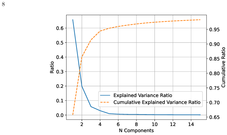
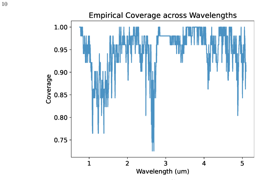
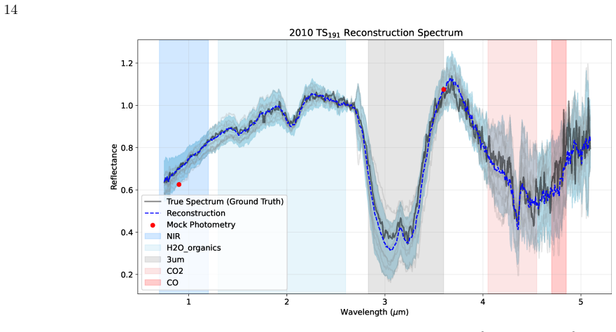
Using a principal component representation trained on a sample of near-IR spectra, we model the spectral manifold of TNOs and perform Bayesian inference in this reduced space to reconstruct full spectra from photometry while propagating uncertainties. Leave-one-out cross-validation demonstrates that the dominant modes of spectral variability are low-dimensional: 4 to 5 principal components capture the structure relevant for taxonomic classification, while 8-10 components improve spectral reconstruction fidelity and uncertainty calibration. For most objects, the reconstructed spectra achieve empirical credible-interval coverage of 95 percent across wavelength. This suggests the diversity of近红
What carries the argument
Principal component analysis trained on near-IR spectra, enabling Bayesian inference in the reduced latent space to reconstruct spectra from photometry.
Load-bearing premise
The training sample of near-IR spectra is representative of the full diversity of TNO spectral shapes.
What would settle it
Full spectroscopy of an object whose photometry-based reconstruction lies outside the reported 95 percent credible intervals across wavelengths would contradict the coverage result.
Figures


read the original abstract
Near-infrared (near-IR) spectroscopy provides critical constraints on the surface composition of trans-Neptunian objects (TNOs), but spectroscopic observations remain limited compared to broadband photometry. We develop a probabilistic latent-space framework to quantify how much spectral information is retained in sparse photometric measurements. Using a principal component representation trained on a sample of near-IR spectra, we model the spectral manifold of TNOs and perform Bayesian inference in this reduced space to reconstruct full spectra from photometry while propagating uncertainties. Leave-one-out cross-validation demonstrates that the dominant modes of spectral variability are low-dimensional: 4 to 5 principal components capture the structure relevant for taxonomic classification, while 8-10 components improve spectral reconstruction fidelity and uncertainty calibration. For most objects, the reconstructed spectra achieve empirical credible-interval coverage of 95 percent across wavelength. This suggests the diversity of near-IR spectral shapes is governed by structured, correlated surface processes rather than stochastic variation. Practically, we apply this framework to survey optimization, quantifying the information content of JWST/NIRCam filters to identify optimal configurations (e.g., F090W, F115W, F410M, F460M) for TNO taxonomy. Additionally, we demonstrate the pipeline's capability to detect and reconstruct rare spectral types, such as the peculiar Neptune Trojans 2006 RJ103 and 2011 SO277, by allowing constraining photometry to select low-probability intermediate models from the continuous topological manifold. Ultimately, this framework bridges the gap between sparse photometry and spectroscopy, providing a statistically rigorous tool to map the compositional structure of minor planets in upcoming large-scale surveys.
Editorial analysis
A structured set of objections, weighed in public.
Referee Report
Summary. The paper develops a probabilistic latent-space framework for reconstructing near-IR spectra of trans-Neptunian objects from sparse photometry. It trains PCA on a sample of near-IR spectra to define a low-dimensional manifold, then performs Bayesian inference over the PCA coefficients given photometric constraints while propagating uncertainties. Leave-one-out cross-validation on the training spectra is used to argue that 4-5 principal components suffice for taxonomy and 8-10 yield 95% empirical credible-interval coverage; the framework is further applied to JWST/NIRCam filter optimization and to outlier reconstruction for two Neptune Trojans.
Significance. If externally validated, the approach would provide a statistically grounded way to extract spectral information from the much larger photometric datasets expected from LSST and other surveys, while highlighting the low-dimensional structure of TNO spectral variability. The filter-optimization results and outlier-handling capability are practically useful, but the strength of these claims depends on whether the PCA basis generalizes beyond the training spectra.
major comments (3)
- [Results on LOO CV and spectral reconstruction] The leave-one-out cross-validation (reported in the results section on dimensionality and coverage) holds out spectra that were already used to construct the PCA basis. This internal validation cannot confirm that the Bayesian posterior over PCA coefficients remains well-calibrated when applied to photometry of TNOs whose near-IR spectral shapes lie outside the training manifold, which is load-bearing for the reconstruction-fidelity and 95% coverage claims.
- [Methods on PCA training and data sample] The representativeness assumption for the training spectral sample is stated but not tested with external data or selection-effect analysis. No quantitative assessment of how well the sampled TNOs cover compositional or orbital phase space is provided, directly affecting whether the reported dimensionality (4-5 PCs for taxonomy) and uncertainty calibration generalize to new objects.
- [Application to outlier detection] The two Neptune Trojan examples (2006 RJ103 and 2011 SO277) are presented as demonstrations of outlier detection via the continuous manifold, but two cases do not constitute a systematic external test of generalization or robustness to objects with rare spectral types.
minor comments (2)
- [Data and methods] Clarify the precise number of spectra in the training set and any cuts applied (e.g., wavelength coverage, S/N thresholds) so readers can assess sample size relative to the number of retained principal components.
- [Survey optimization results] In the JWST filter-optimization discussion, explicitly state the assumed photometric uncertainties and how they propagate into the information-content metric.
Simulated Author's Rebuttal
We thank the referee for the constructive comments on our manuscript. We agree that the validation aspects require clarification regarding the scope of the claims. We will revise the paper to better articulate the limitations of the internal validation and the representativeness of the training sample, while reframing the outlier examples as illustrative. Our responses to each major comment are provided below.
read point-by-point responses
-
Referee: The leave-one-out cross-validation (reported in the results section on dimensionality and coverage) holds out spectra that were already used to construct the PCA basis. This internal validation cannot confirm that the Bayesian posterior over PCA coefficients remains well-calibrated when applied to photometry of TNOs whose near-IR spectral shapes lie outside the training manifold, which is load-bearing for the reconstruction-fidelity and 95% coverage claims.
Authors: We acknowledge that the leave-one-out cross-validation provides an internal assessment within the training spectral sample and does not directly test generalization to spectra outside the observed manifold. The 95% credible interval coverage is an empirical result for the held-out training spectra. For new TNOs, if their spectral shapes fall outside the training distribution, the model may underperform, which the framework can flag through elevated reconstruction uncertainties or outlier probabilities. In the revised manuscript, we will add explicit language in the results and discussion sections stating that the coverage claims apply to objects consistent with the training distribution and discuss the implications for applying the method to the broader TNO population. This revision will strengthen the manuscript by transparently addressing the generalization limits. revision: partial
-
Referee: The representativeness assumption for the training spectral sample is stated but not tested with external data or selection-effect analysis. No quantitative assessment of how well the sampled TNOs cover compositional or orbital phase space is provided, directly affecting whether the reported dimensionality (4-5 PCs for taxonomy) and uncertainty calibration generalize to new objects.
Authors: The training sample is limited to the available published near-IR spectra of TNOs, which we acknowledge may not fully represent the entire population due to observational biases toward brighter or more accessible objects. We agree that a quantitative assessment of coverage is warranted. In the revised version, we will include an analysis of the orbital parameter space (e.g., semi-major axis vs. inclination) covered by the training objects compared to the known TNO catalog, along with a discussion of potential selection effects. This will provide readers with a better understanding of the sample's representativeness. However, performing a full external validation would require additional independent spectra, which are not currently available in sufficient numbers. revision: yes
-
Referee: The two Neptune Trojan examples (2006 RJ103 and 2011 SO277) are presented as demonstrations of outlier detection via the continuous manifold, but two cases do not constitute a systematic external test of generalization or robustness to objects with rare spectral types.
Authors: We concur that two specific cases do not amount to a systematic test of the outlier detection capability. These examples were intended to demonstrate how the continuous manifold allows reconstruction of intermediate spectral types for objects that deviate from the primary modes. In the revised manuscript, we will modify the relevant section to present these as illustrative case studies of the framework's application to potential outliers, rather than as validation of the method's robustness. We will also note that systematic testing would benefit from larger photometric samples expected from future surveys like LSST. revision: yes
Circularity Check
No circularity in derivation chain
full rationale
The framework trains PCA on an external near-IR spectral sample, performs Bayesian inference over latent coefficients given photometry, and reports LOO cross-validation results on held-out members of that same sample. No equation reduces a claimed output (e.g., 4–5 PCs for taxonomy or 95 % coverage) to a fitted quantity by construction, nor does any load-bearing premise rest on a self-citation whose content is itself unverified. The derivation remains self-contained against the external spectral training data and the photometric observations to which the model is applied.
Axiom & Free-Parameter Ledger
free parameters (1)
- Number of principal components =
4-5 or 8-10
axioms (2)
- domain assumption TNO near-IR spectral variability is captured by a low-dimensional linear manifold via PCA.
- domain assumption Photometric measurements provide sufficient constraints to perform inference in the latent space.
invented entities (1)
-
Continuous topological manifold of TNO spectra
no independent evidence
Reference graph
Works this paper leans on
-
[1]
Fast likelihood-free cosmology with neural density estimators and active learning , ISSN=
Alsing, J., Charnock, T., Feeney, S., & Wandelt, B. 2019, MNRAS, 488, 4440, doi: 10.1093/mnras/stz1960
-
[2]
Alsing, J., Wandelt, B., & Feeney, S. 2018, MNRAS, 477, 2874, doi: 10.1093/mnras/sty819 Arsalan Bashir, S. M., Wang, Y., Khan, M., & Niu, Y. 2021, arXiv e-prints, arXiv:2102.09351, doi: 10.48550/arXiv.2102.09351 Astropy Collaboration, Robitaille, T. P., Tollerud, E. J., et al. 2013, A&A, 558, A33, doi: 10.1051/0004-6361/201322068 Astropy Collaboration, Pr...
-
[3]
Barucci, M. A., Belskaya, I. N., Fulchignoni, M., & Birlan, M. 2005, AJ, 130, 1291, doi: 10.1086/431957
-
[4]
R., Milby, Z., Wong, I., & Brown, M
Belyakov, M., Davis, M. R., Milby, Z., Wong, I., & Brown, M. E. 2024, PSJ, 5, 119, doi: 10.3847/PSJ/ad3d55
-
[5]
Bernardinelli, P. H., Bernstein, G. M., Jindal, N., et al. 2023, ApJS, 269, 18, doi: 10.3847/1538-4365/acf6bf
-
[6]
Bernardinelli, P. H., Bernstein, G. M., Abbott, T. M. C., et al. 2025, AJ, 169, 305, doi: 10.3847/1538-3881/adc459
-
[7]
Bizhani, M., Ardakani, O. H., & Little, E. 2022, Scientific Reports, 12, 4264, doi: 10.1038/s41598-022-08170-8
-
[8]
2019 b , , 874, 106, 10.3847/1538-4357/ab06c1
Brout, D., Sako, M., Scolnic, D., et al. 2019, ApJ, 874, 106, doi: 10.3847/1538-4357/ab06c1
-
[9]
A., Dotto, E., & Strazzulla, G
Brunetto, R., Barucci, M. A., Dotto, E., & Strazzulla, G. 2006, ApJ, 644, 646, doi: 10.1086/503359
-
[10]
2025, ApJL, 982, L8, doi: 10.3847/2041-8213/adb977
Brunetto, R., Hénault, E., Cryan, S., et al. 2025, ApJL, 982, L8, doi: 10.3847/2041-8213/adb977
-
[11]
Bus, S. J., & Binzel, R. P. 2002a, Icarus, 158, 106, doi: 10.1006/icar.2002.6857
-
[12]
Bus, S. J., & Binzel, R. P. 2002b, Icarus, 158, 146, doi: 10.1006/icar.2002.6856
-
[13]
2023, JWST Calibration Pipeline, 1.11.4 Zenodo, doi: 10.5281/zenodo.8247246 24
Bushouse, H., Eisenhamer, J., Dencheva, N., et al. 2023, JWST Calibration Pipeline, 1.11.4 Zenodo, doi: 10.5281/zenodo.8247246 24
-
[14]
XGBoost: A Scalable Tree Boosting System
Chen, T., & Guestrin, C. 2016, in Proceedings of the 22nd ACM SIGKDD International Conference on Knowledge Discovery and Data Mining (ACM), 785–794, doi: 10.1145/2939672.2939785
-
[15]
Cruikshank, D. P., Moroz, L. V., & Clark, R. N. 2019, Spectroscopy of Ices, Volatiles, and Organics in the Visible and Infrared Regions, ed. J. L. Bishop, I. Bell, James F., & J. E. Moersch, 102–119, doi: 10.1017/9781316888872.007 Dalle Ore, C. M., Barucci, M. A., Emery, J. P., et al. 2015, Icarus, 252, 311, doi: 10.1016/j.icarus.2015.01.014
-
[16]
Delbo, M., Dyer, T., Bhat, U., et al. 2026, Gaia DR3 supervised classification of asteroid reflectance spectra, https://arxiv.org/abs/2602.22816
-
[17]
DeMeo, F. E., Binzel, R. P., Slivan, S. M., & Bus, S. J. 2009, Icarus, 202, 160, doi: 10.1016/j.icarus.2009.02.005
-
[18]
DeMeo, F. E., & Carry, B. 2013, Icarus, 226, 723, doi: 10.1016/j.icarus.2013.06.027
-
[19]
DeMeo, F. E., & Carry, B. 2014, Nature, 505, 629, doi: 10.1038/nature12908
-
[20]
P., Wong, I., Brunetto, R., et al
Emery, J. P., Wong, I., Brunetto, R., et al. 2024, Icarus, 414, 116017, doi: 10.1016/j.icarus.2024.116017
-
[21]
AutoGluon-Tabular: Robust and Accurate AutoML for Structured Data
Erickson, N., Mueller, J., Shirkov, A., et al. 2020, arXiv preprint arXiv:2003.06505
work page internal anchor Pith review arXiv 2020
-
[22]
Fraser, W. C., Pike, R. E., Marsset, M., et al. 2023, PSJ, 4, 80, doi: 10.3847/PSJ/acc844
-
[23]
He, K., Chen, X., Xie, S., et al. 2022, in 2022 IEEE/CVF Conference on Computer Vision and Pattern Recognition (CVPR), 15979–15988, doi: 10.1109/CVPR52688.2022.01553 Hénault, E., Brunetto, R., Pinilla-Alonso, N., et al. 2025, A&A, 694, A126, doi: 10.1051/0004-6361/202452321
-
[24]
Data analysis recipes: Fitting a model to data
Hogg, D. W., Bovy, J., & Lang, D. 2010, arXiv e-prints, arXiv:1008.4686, doi: 10.48550/arXiv.1008.4686
-
[25]
J., Brunetto, R., Cruikshank, D
Holler, B. J., Brunetto, R., Cruikshank, D. P., et al. 2025, Research Notes of the American Astronomical Society, 9, 241, doi: 10.3847/2515-5172/ae03a2
-
[26]
Huang, J.-B., Singh, A., & Ahuja, N. 2015, in 2015 IEEE Conference on Computer Vision and Pattern Recognition (CVPR), 5197–5206, doi: 10.1109/CVPR.2015.7299156 Ivezić, Ž., Connolly, A. J., VanderPlas, J. T., & Gray, A. 2014, Statistics, Data Mining, and Machine Learning in Astronomy: A Practical Python Guide for the Analysis of Survey Data, doi: 10.1515/9...
-
[27]
Jeffrey, N., Alsing, J., & Lanusse, F. 2021, MNRAS, 501, 954, doi: 10.1093/mnras/staa3594
-
[28]
Licandro, J., Pinilla-Alonso, N., Holler, B. J., et al. 2025, Nature Astronomy, 9, 245, doi: 10.1038/s41550-024-02417-2
-
[29]
2024, AJ, 167, 13, doi: 10.3847/1538-3881/ad0b7a
Luo, N., Wang, X., Gu, S., et al. 2024, AJ, 167, 13, doi: 10.3847/1538-3881/ad0b7a
-
[30]
Markwardt, L., Lin, H. W., Holler, B. J., et al. 2025, PSJ, 6, 154, doi: 10.3847/PSJ/addecd Nesvorný, D., Vokrouhlický, D., Alexand ersen, M., et al. 2020, AJ, 160, 46, doi: 10.3847/1538-3881/ab98fb
-
[31]
2011, Journal of Machine Learning Research, 12, 2825
Pedregosa, F., Varoquaux, G., Gramfort, A., et al. 2011, Journal of Machine Learning Research, 12, 2825
2011
-
[32]
2015, A&A, 577, A35, doi: 10.1051/0004-6361/201425436
Peixinho, N., Delsanti, A., & Doressoundiram, A. 2015, A&A, 577, A35, doi: 10.1051/0004-6361/201425436
-
[33]
2012, A&A, 546, A86, doi: 10.1051/0004-6361/201219057 Penttilä, A., Fedorets, G., & Muinonen, K
Peixinho, N., Delsanti, A., Guilbert-Lepoutre, A., Gafeira, R., & Lacerda, P. 2012, A&A, 546, A86, doi: 10.1051/0004-6361/201219057 Penttilä, A., Fedorets, G., & Muinonen, K. 2022, Frontiers in Astronomy and Space Sciences, 9, 816268, doi: 10.3389/fspas.2022.816268 Penttilä, A., Hietala, H., & Muinonen, K. 2021, A&A, 649, A46, doi: 10.1051/0004-6361/202038545
-
[34]
Pike, R. E., Fraser, W. C., Schwamb, M. E., et al. 2017, AJ, 154, 101, doi: 10.3847/1538-3881/aa83b1
-
[35]
Pinilla-Alonso, N., Brunetto, R., De Prá, M. N., et al. 2025, Nature Astronomy, 9, 230, doi: 10.1038/s41550-024-02433-2
-
[36]
Schwamb, M. E., Fraser, W. C., Bannister, M. T., et al. 2019, ApJS, 243, 12, doi: 10.3847/1538-4365/ab2194 Souza Feliciano, A. C., Holler, B., Grundy, W., et al. 2025, in EPSC-DPS Joint Meeting 2025, Vol. 2025, EPSC–DPS2025–848, doi: 10.5194/epsc-dps2025-848
-
[37]
A., Fraser, W
Stansberry, J. A., Fraser, W. C., Trilling, D. E., et al. 2021, An Ultra-Sensitive Pencil Beam Search for 10 km Trans-Neptunian Objects„ JWST Proposal. Cycle 1, ID. #1568
2021
- [38]
-
[39]
Tai, Y.-W., Liu, S., Brown, M. S., & Lin, S. 2010, in 2010 IEEE Computer Society Conference on Computer Vision and Pattern Recognition, 2400–2407, doi: 10.1109/CVPR.2010.5539933
-
[40]
2025, AJ, 169, 201, doi: 10.3847/1538-3881/adb710
Tang, Y., Jiang, Y., Feng, Y., Zhang, X., & Jiang, X. 2025, AJ, 169, 201, doi: 10.3847/1538-3881/adb710
-
[41]
1987, Inverse problem theory
Tarantola, A. 1987, Inverse problem theory. Methods for data fitting and model parameter estimation
1987
-
[42]
Tegler, S. C., & Romanishin, W. 1998, Nature, 392, 49, doi: 10.1038/32108
-
[43]
Tsiganis, K., Gomes, R., Morbidelli, A., & Levison, H. F. 2005, Nature, 435, 459, doi: 10.1038/nature03539
-
[44]
2017, in Super-Resolution Imaging (CRC Press), 155–186
Vandewalle, P., Sbaiz, L., & Vetterli, M. 2017, in Super-Resolution Imaging (CRC Press), 155–186
2017
-
[45]
Virtanen, P., Gommers, R., Oliphant, T. E., et al. 2020, Nature Methods, 17, 261, doi: 10.1038/s41592-019-0686-2
-
[46]
2015, Deep Networks for Image Super-Resolution with Sparse Prior, https://arxiv.org/abs/1507.08905
Wang, Z., Liu, D., Yang, J., Han, W., & Huang, T. 2015, Deep Networks for Image Super-Resolution with Sparse Prior, https://arxiv.org/abs/1507.08905
-
[47]
Wong, I., Holler, B. J., Fraser, W. C., & Brown, M. E. 2025, PSJ, 6, 271, doi: 10.3847/PSJ/ae1d73
-
[48]
Star: A benchmark for astronomical star fields super-resolution.arXiv preprint arXiv:2507.16385,
Wu, K.-C., Zhuang, G., Huang, J., et al. 2025, STAR: A Benchmark for Astronomical Star Fields Super-Resolution, https://arxiv.org/abs/2507.16385
-
[49]
Xu, S., Binzel, R. P., Burbine, T. H., & Bus, S. J. 1995, Icarus, 115, 1, doi: 10.1006/icar.1995.1075
-
[50]
Zhang, C., Zhu, C., Turner, A. M., et al. 2023, Science Advances, 9, eadg6936, doi: 10.1126/sciadv.adg6936
discussion (0)
Sign in with ORCID, Apple, or X to comment. Anyone can read and Pith papers without signing in.