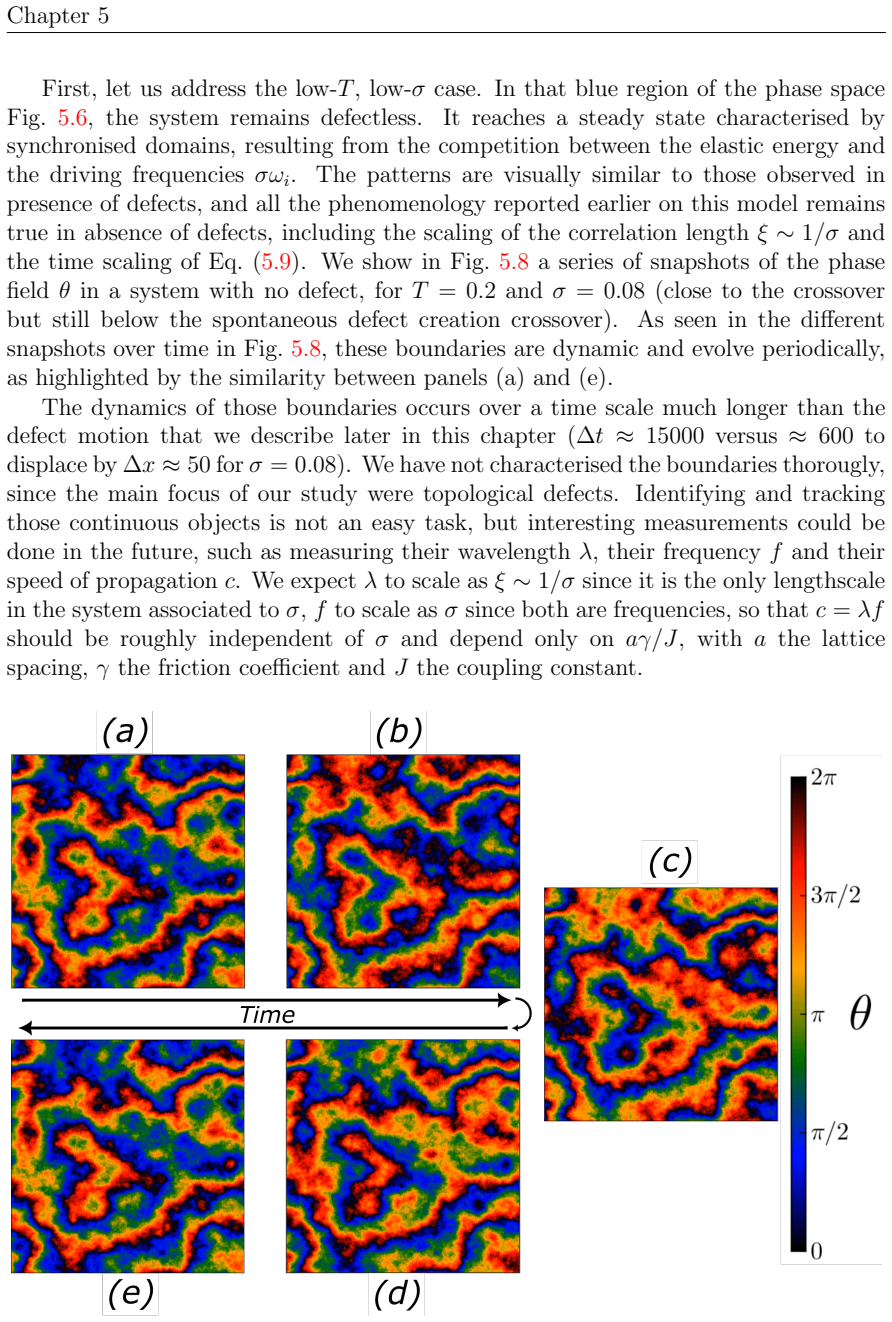
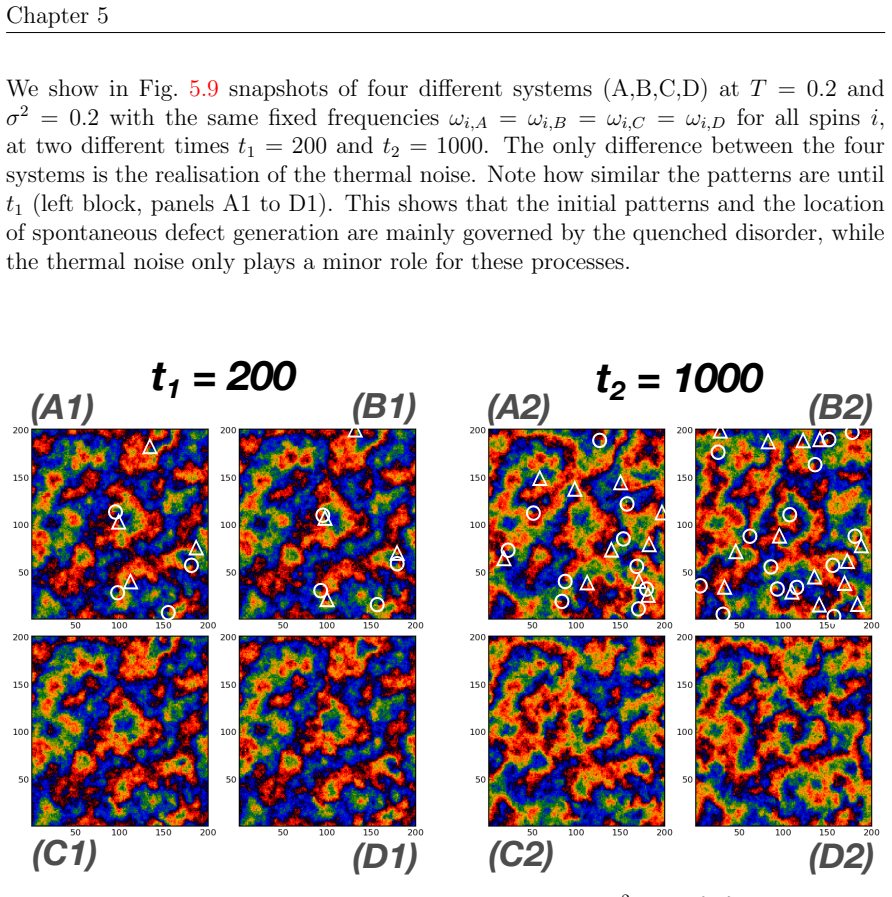
Recognition: 3 theorem links
· Lean TheoremTopological defects in out-of-equilibrium systems
Pith reviewed 2026-05-08 18:02 UTC · model grok-4.3
The pith
Allowing oscillators to move restores quasi-long-range order through a Berezinskii-Kosterlitz-Thouless transition despite frequency heterogeneity.
A machine-rendered reading of the paper's core claim, the machinery that carries it, and where it could break.
Core claim
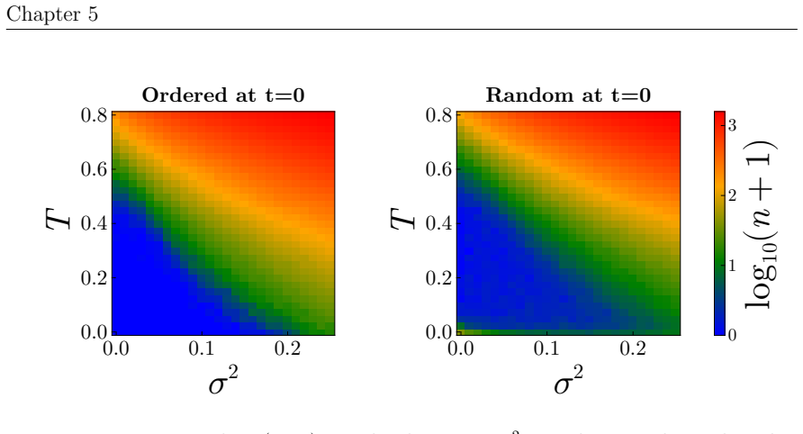
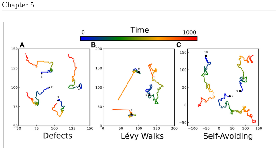
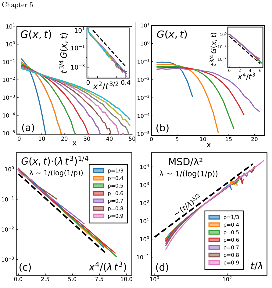
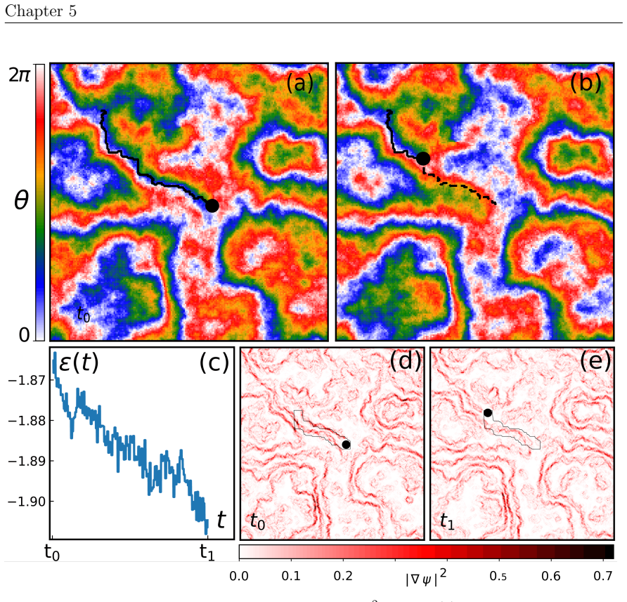
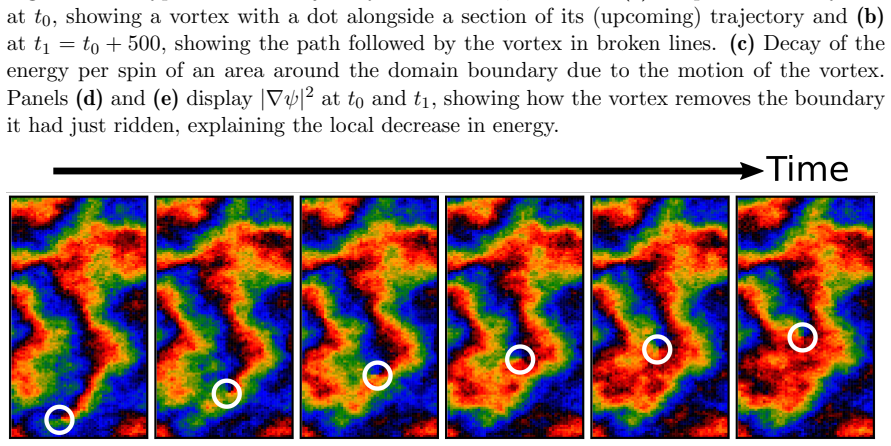
In a noisy Kuramoto lattice with short-range coupling, intrinsic frequency heterogeneity destroys quasi-long-range order and fragments the system into finite domains where defects unbind at all temperatures and follow superdiffusive random walks advected by evolving boundaries. By contrast, when oscillators are allowed to move in space the system undergoes a Berezinskii-Kosterlitz-Thouless transition and regains quasi-long-range order. In the non-reciprocal O(2) model with vision-cone couplings, the derived continuum theory shows that non-reciprocity selects defect shapes, enriches the annihilation process, and reshapes patterns through advection.
What carries the argument
Motility of oscillators in the active XY lattice, which enables a Berezinskii-Kosterlitz-Thouless transition that binds vortex defects and restores algebraic order.
Load-bearing premise
The continuum theory derived for the non-reciprocal model accurately reproduces the large-scale defect motion and annihilation seen in the underlying discrete lattice without hidden parameters or approximations that alter those dynamics.
What would settle it
A direct simulation or experiment in which oscillators with heterogeneous frequencies are allowed to move and either shows persistent unbound defects at all temperatures or a clear transition to bound defects and algebraic order below a critical motility threshold.
Figures


read the original abstract
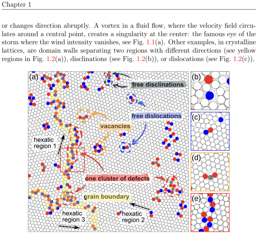
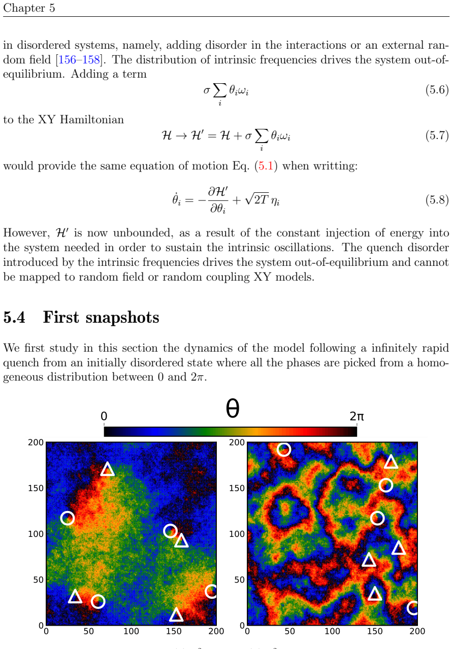
In this PhD thesis, we study topological defects in two-dimensional non-equilibrium systems, focusing on active extensions of the XY model, including activity, mobility and non-reciprocity. In a noisy Kuramoto lattice with short-range coupling, intrinsic frequency heterogeneity destroys quasi-long-range order and fragments the system into finite domains. Defects unbind at all temperatures and exhibit superdiffusive random walks, advected by evolving domain boundaries. By contrast, when oscillators are allowed to move in space, the system undergoes a Berezinskii-Kosterlitz-Thouless transition and regains quasi-long-range order, revealing the fundamental role of motility in sustaining coherence. We also analyse a non-reciprocal O(2) model with vision-cone couplings and derive a continuum theory that captures the same large-scale physics. Non-reciprocity selects defect shapes, enriches the annihilation process, and reshapes patterns through advection. Together, these results elucidate the fundamental role of activity and non-reciprocity in shaping topological defects and ordering in non-equilibrium systems. Keywords: Topological defects, XY model, Steep XY model, Kuramoto model, Non-reciprocal interactions, Active matter, Phase transitions, Berezinskii-Kosterlitz-Thouless transition, Non-equilibrium statistical mechanics
Editorial analysis
A structured set of objections, weighed in public.
Referee Report
Summary. The manuscript is a PhD thesis studying topological defects in two-dimensional non-equilibrium systems, with focus on active extensions of the XY/Kuramoto model that incorporate activity, mobility, and non-reciprocity. In a noisy Kuramoto lattice with short-range coupling, intrinsic frequency heterogeneity destroys quasi-long-range order, fragments the system into finite domains, and produces superdiffusive defect walks advected by domain boundaries. Allowing oscillators to move spatially restores a Berezinskii-Kosterlitz-Thouless transition and quasi-long-range order. A non-reciprocal O(2) model with vision-cone couplings is also analyzed; a continuum theory is derived that reproduces the large-scale physics, with non-reciprocity selecting defect shapes, enriching annihilation, and driving advection-induced pattern reshaping.
Significance. If the central claims hold, the work establishes motility as a key mechanism for sustaining coherence and quasi-long-range order in active oscillator systems, extending the BKT framework to non-equilibrium settings with non-reciprocal interactions. Strengths include direct lattice simulations of defect dynamics and the explicit derivation of hydrodynamic equations from microscopic rules, which together provide falsifiable predictions for defect advection and annihilation rates.
major comments (2)
- [Continuum theory derivation] Continuum theory derivation (vision-cone non-reciprocal O(2) model): the claim that the hydrodynamic equations faithfully reproduce discrete-lattice defect advection and annihilation requires an explicit parameter mapping and a quantitative check that predicted defect-density scaling matches lattice data. Without this, higher-order correlations between defect positions and the local velocity field could alter the effective core energy or renormalized stiffness, converting a true BKT transition into a crossover.
- [Motility and BKT restoration] Motility and BKT restoration section: the assertion that spatial mobility restores the BKT transition and quasi-long-range order rests on numerical evidence whose details (how the continuum limit is taken, error bars on defect densities, and the precise diagnostic for the transition such as helicity modulus jump or defect-unbinding criterion) are not yet sufficient to rule out finite-size or post-hoc interpretation effects.
minor comments (2)
- Abstract and introduction should explicitly state the microscopic parameters (coupling strength, noise amplitude, motility speed) used in the lattice simulations so that the continuum coefficients can be directly compared.
- Figure captions for defect trajectories and density plots should include the system size, averaging procedure, and how the superdiffusive exponent is extracted.
Simulated Author's Rebuttal
We thank the referee for their careful reading of the manuscript and for the constructive comments, which help clarify the presentation of our results on topological defects in active oscillator systems. We address each major comment point by point below.
read point-by-point responses
-
Referee: [Continuum theory derivation] Continuum theory derivation (vision-cone non-reciprocal O(2) model): the claim that the hydrodynamic equations faithfully reproduce discrete-lattice defect advection and annihilation requires an explicit parameter mapping and a quantitative check that predicted defect-density scaling matches lattice data. Without this, higher-order correlations between defect positions and the local velocity field could alter the effective core energy or renormalized stiffness, converting a true BKT transition into a crossover.
Authors: We agree that an explicit parameter mapping and quantitative validation would strengthen the link between the microscopic lattice model and the derived hydrodynamic equations. In the revised manuscript we will add a dedicated subsection providing the full parameter mapping (including how microscopic coupling strengths, vision-cone angles, and noise amplitudes translate to continuum coefficients) together with a direct numerical comparison of defect-density scaling between lattice simulations and the continuum theory, including ensemble error bars. This addition will also allow us to discuss the possible influence of higher-order correlations on core energies and stiffness renormalization. revision: yes
-
Referee: [Motility and BKT restoration] Motility and BKT restoration section: the assertion that spatial mobility restores the BKT transition and quasi-long-range order rests on numerical evidence whose details (how the continuum limit is taken, error bars on defect densities, and the precise diagnostic for the transition such as helicity modulus jump or defect-unbinding criterion) are not yet sufficient to rule out finite-size or post-hoc interpretation effects.
Authors: We appreciate the referee’s request for greater transparency in the numerical diagnostics. The BKT transition is diagnosed via the universal jump in the helicity modulus and the associated unbinding of defect pairs, with defect densities averaged over independent realizations and shown with error bars. The continuum limit is approached by increasing linear system size at fixed oscillator density while monitoring finite-size scaling of the helicity modulus. In the revision we will expand the methods and results sections to include explicit descriptions of these procedures, additional finite-size scaling plots, and a clear statement of the defect-unbinding criterion used, thereby addressing concerns about post-hoc interpretation and finite-size effects. revision: yes
Circularity Check
No circularity: results rest on lattice simulations and independent continuum derivation.
full rationale
The abstract and available text describe direct numerical results on the noisy Kuramoto lattice (defect unbinding, superdiffusion, domain advection) and the motility extension that restores BKT order, plus a separate derivation of hydrodynamic equations for the vision-cone non-reciprocal O(2) model. No quoted equations, parameter fits, or self-citations are shown that would make any prediction equivalent to its input by construction. The continuum theory is presented as capturing the same large-scale physics without evidence of closure assumptions that tautologically enforce the claimed advection or annihilation behaviors. This is the common honest case of a self-contained derivation chain.
Axiom & Free-Parameter Ledger
axioms (1)
- domain assumption Standard assumptions of the two-dimensional XY model and Kuramoto oscillator lattice for describing phase ordering and synchronization.
Lean theorems connected to this paper
-
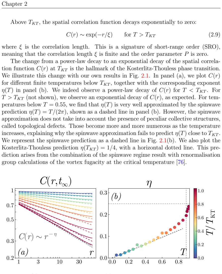
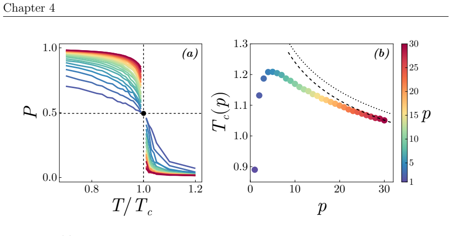
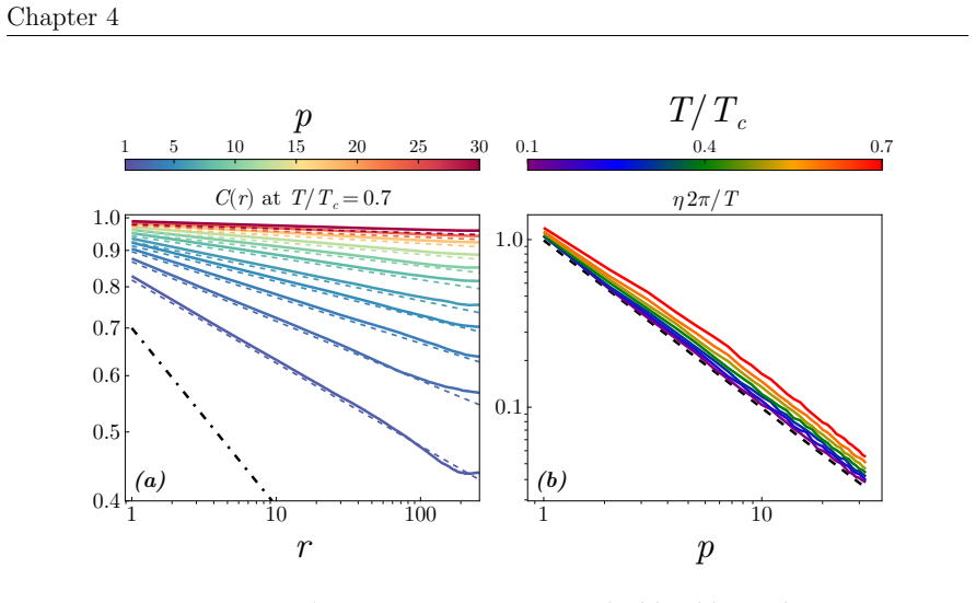
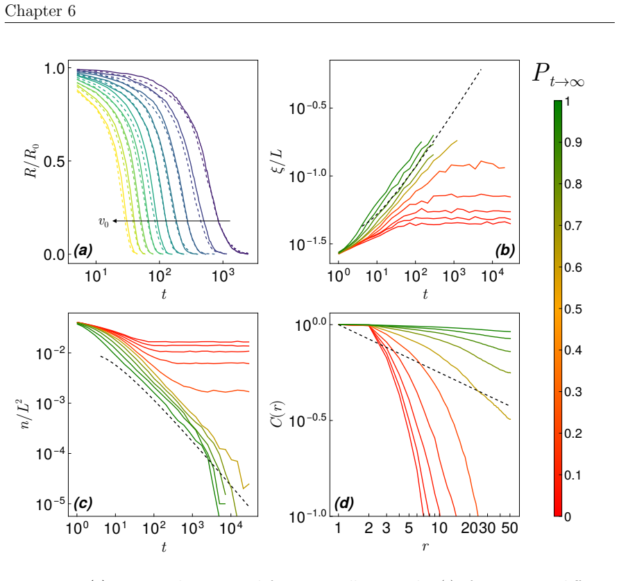
Foundation/AlexanderDuality.lean (RS pins D=3 via circle-linking; paper fixes D=2 by modeling choice — different domain)alexander_duality_circle_linking unclearThe XY model... undergoes a topological phase transition, known as the Kosterlitz-Thouless (KT) phase transition... characterised by a sudden change in the asymptotic behaviour of the equal-time spatial correlation function C(r,t)... C(r) ∼ r^{-η(T)} for T<T_KT
-
Cost/FunctionalEquation.lean (RS's J(x)=½(x+x⁻¹)−1 cost-forcing is absent in the paper's energy)washburn_uniqueness_aczel unclearHamiltonian H = -J Σ cos(θ_i − θ_j); Langevin dynamics; Peierls argument F = (Jπq² − 2k_B T) log(L/a)
Reference graph
Works this paper leans on
-
[1]
Self-propelled rods: Insights and perspectives for active matter.Annu
Markus B ¨ar, Robert Großmann, Sebastian Heidenreich, and Fernando Peruani. Self-propelled rods: Insights and perspectives for active matter.Annu. Rev. Condens. Matter Phys., 11:441–466, 2020
2020
-
[2]
Noise-aware neural network for stochastic dynamics simulation.arXiv preprint arXiv:2403.09370, 2024
Pei-Fang Wu, Wei-Chen Guo, and Liang He. Noise-aware neural network for stochastic dynamics simulation.arXiv preprint arXiv:2403.09370, 2024
-
[3]
Uncertainty in ai-driven monte carlo simulations.arXiv preprint arXiv:2506.14594, 2025
Dimitrios Tzivrailis, Alberto Rosso, and Eiji Kawasaki. Uncertainty in ai-driven monte carlo simulations.arXiv preprint arXiv:2506.14594, 2025
-
[4]
Ruslan Mukhamadiarov. Controlling dynamics of stochastic systems with deep reinforcement learning.arXiv preprint arXiv:2502.18111, 2025
-
[5]
Discovering governing equations from data by sparse identification of nonlinear dynamical systems
Steven L Brunton, Joshua L Proctor, and J Nathan Kutz. Discovering governing equations from data by sparse identification of nonlinear dynamical systems. Proc. Natl. Acad. Sci., 113(15):3932–3937, 2016
2016
-
[6]
Interpreting neural operators: How nonlinear waves propagate in nonreciprocal solids.Phys
Jonathan Colen, Alexis Poncet, Denis Bartolo, and Vincenzo Vitelli. Interpreting neural operators: How nonlinear waves propagate in nonreciprocal solids.Phys. Rev. Lett., 133(10):107301, 2024
2024
-
[7]
Yi-Lun Du, Nan Su, and Konrad Tywoniuk. Discovering novel order parameters in the potts model: A bridge between machine learning and critical phenomena. arXiv preprint arXiv:2505.06159, 2025
-
[8]
Machine learning of phase transitions in the percolation and xy models.Phys
Wanzhou Zhang, Jiayu Liu, and Tzu-Chieh Wei. Machine learning of phase transitions in the percolation and xy models.Phys. Rev. E, 99(3):032142, 2019
2019
-
[9]
Machine learning topological defect formation.arXiv preprint arXiv:2508.20347, 2025
Fumika Suzuki, Ying Wai Li, and Wojciech H Zurek. Machine learning topological defect formation.arXiv preprint arXiv:2508.20347, 2025
-
[10]
Variational autoencoders understand knot topology.Phys
Anna Braghetto, Sumanta Kundu, Marco Baiesi, and Enzo Orlandini. Variational autoencoders understand knot topology.Phys. Rev. E, 112(2):025418, 2025
2025
-
[11]
Attention is all you need
Ashish Vaswani, Noam Shazeer, Niki Parmar, Jakob Uszkoreit, Llion Jones, Aidan N Gomez, Lukasz Kaiser, and Illia Polosukhin. Attention is all you need. Adv. Neural Inf. Process. Syst., 30, 2017
2017
-
[12]
First language acquisition.The handbook of linguistics, pages 397–413, 2017
Brian MacWhinney. First language acquisition.The handbook of linguistics, pages 397–413, 2017. PhD Thesis in Physics Topological defects in out-of-equilibrium systems Author:Ylann Rouzaire PhD Supervisors:Demian Levis and Ignacio Pagonabarraga We study topological defects in two-dimensional non-equilibrium systems, focusing on active extensions of the XY ...
2017
discussion (0)
Sign in with ORCID, Apple, or X to comment. Anyone can read and Pith papers without signing in.