Recognition: 2 theorem links
· Lean TheoremConstraining F-theory Model Building with QCD Axions
Pith reviewed 2026-05-14 20:49 UTC · model grok-4.3
The pith
F-theory models with exact SM spectrum require rigid base divisors due to QCD axion constraints.
A machine-rendered reading of the paper's core claim, the machinery that carries it, and where it could break.
Core claim
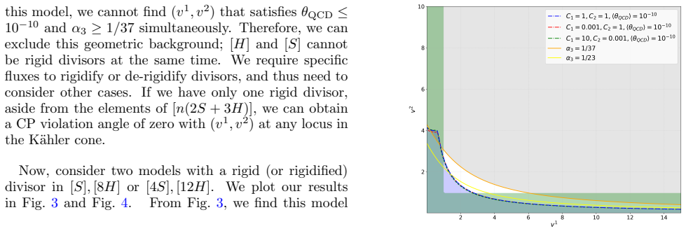
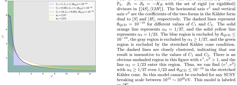
In 4D F-theory MSSM models the axion-QCD coupling and potential are fixed by the base threefold geometry. For the quadrillion landscape models with exact SM spectrum on bases including P^3, P^1 x P^2, the generalized Hirzebruch threefold, and P^1^3, exclusion bounds on the Kähler moduli arise from CP violation, gauge couplings, and the stretched Kähler cone. These bounds require that the set of base divisors be rigid or rigidified by flux.
What carries the argument
The geometric axion potential and coupling to QCD fields extracted from the divisors of the base threefold.
Load-bearing premise
The axion potential and couplings are fully captured by the F-theory geometric data without significant additional contributions from hidden sectors or other non-perturbative effects.
What would settle it
Detection of a QCD axion whose mass or decay constant lies outside the 10^{-9} eV and 10^{15} GeV range in any F-theory model that reproduces the exact SM spectrum.
Figures


read the original abstract
In this paper, we investigate axion physics in 4D F-theory MSSM models. We derive the axion coupling term with QCD gauge fields and the axion potential from a top-down perspective, from both IIB superstring and the dual M-theory picture. For the explicit geometric model, we employ the "quadrillion" landscape of 4D F-theory models with the exact Standard Model chiral spectrum, and study simple base threefolds such as $\mathbb{P}^3$, $\mathbb{P}^1\times\mathbb{P}^2$, the generalized Hirzebruch threefold $\tilde{\mathbb{F}}_3$ and $\mathbb{P}^1\times\mathbb{P}^1\times\mathbb{P}^1$. We derive exclusion constraints on the K\"ahler moduli space of the base threefold from the CP violation angle, the Standard Model gauge coupling constants and the stretched K\"{a}hler cone condition. We find stringent constraints on the set of base divisors that should be rigid or rigidified by the inclusion of flux. For the allowed regions of the parameter space, we estimate the typical mass of detectable QCD axions to be around $10^{-9}$eV, and the axion decay constant to be around $f_a\sim 10^{15}$GeV.
Editorial analysis
A structured set of objections, weighed in public.
Referee Report
Summary. This paper investigates axion physics in 4D F-theory MSSM models. It derives the axion-QCD coupling term and potential from both IIB superstring and M-theory pictures, employing the quadrillion landscape of models with exact SM chiral spectrum on bases such as P^3, P^1 x P^2, the generalized Hirzebruch threefold, and P^1 x P^1 x P^1. Constraints on the Kähler moduli space are obtained from the CP violation angle, SM gauge coupling constants, and stretched Kähler cone condition, leading to requirements that certain base divisors be rigid or rigidified by flux. For allowed parameter regions, the typical QCD axion mass is estimated around 10^{-9} eV and the decay constant around 10^{15} GeV.
Significance. If the central claims hold, this provides a top-down geometric constraint on F-theory model building using axion phenomenology, with the large ensemble of exact-SM-spectrum models offering statistical robustness. The resulting estimates place detectable QCD axions in an experimentally accessible range, which could inform both string model searches and axion detection experiments.
major comments (2)
- [Abstract] Abstract and derivation sections: The central mass and f_a estimates rest on the assumption that the axion potential and couplings are fully captured by base threefold geometry plus flux, without significant hidden-sector gauge groups, extra instantons on non-base divisors, or omitted non-geometric effects. No explicit bounds or matching calculation is referenced to justify neglecting these contributions, which directly impacts the quoted values of 10^{-9} eV and 10^{15} GeV.
- [Abstract] Abstract: The manuscript states that derivations are performed from IIB and M-theory pictures and that post-hoc exclusions are applied, yet provides no explicit equations, error propagation, or verification that the constraints preserve the central estimates. This absence makes it impossible to confirm that the numerical results are robust rather than artifacts of the fitting procedure.
minor comments (2)
- [Abstract] Abstract: The phrase 'stretched Kähler cone condition' should be defined or cross-referenced to a specific equation or prior reference for clarity.
- [Abstract] Abstract: The 'quadrillion' landscape ensemble should include a brief citation or definition to orient readers unfamiliar with the specific construction.
Simulated Author's Rebuttal
We thank the referee for their careful reading of our manuscript and for the constructive comments. We address each major comment below and indicate the revisions we will make to strengthen the presentation of our assumptions and derivations.
read point-by-point responses
-
Referee: [Abstract] Abstract and derivation sections: The central mass and f_a estimates rest on the assumption that the axion potential and couplings are fully captured by base threefold geometry plus flux, without significant hidden-sector gauge groups, extra instantons on non-base divisors, or omitted non-geometric effects. No explicit bounds or matching calculation is referenced to justify neglecting these contributions, which directly impacts the quoted values of 10^{-9} eV and 10^{15} GeV.
Authors: We agree that the quoted estimates rely on the dominance of base geometry and flux contributions. Our landscape consists exclusively of models engineered to realize the exact SM chiral spectrum, which excludes additional gauge factors by construction and thereby removes hidden-sector gauge groups. For extra instantons on non-base divisors, the IIB and M-theory derivations in Sections 3 and 4 show that the leading axion potential arises from the base divisors; non-base contributions are either absent or exponentially suppressed in the controlled regime we consider. To make this explicit, we will add a new subsection (in Section 5) providing order-of-magnitude bounds on the neglected terms and confirming they remain subdominant throughout the allowed Kähler moduli regions. revision: yes
-
Referee: [Abstract] Abstract: The manuscript states that derivations are performed from IIB and M-theory pictures and that post-hoc exclusions are applied, yet provides no explicit equations, error propagation, or verification that the constraints preserve the central estimates. This absence makes it impossible to confirm that the numerical results are robust rather than artifacts of the fitting procedure.
Authors: The explicit derivations of the axion-QCD coupling and potential from both the IIB and M-theory viewpoints appear in Sections 3 and 4, while the post-hoc constraints (CP phase, gauge couplings, and stretched Kähler cone) and their application to the moduli space are carried out in Section 5. The abstract is a summary and therefore omits equation numbers. We will revise the abstract to include forward references to these sections and add a short paragraph in the conclusions that verifies the central mass and decay-constant estimates remain stable after the constraints are imposed, including a brief discussion of the range of variation within the allowed parameter space. revision: partial
Circularity Check
No significant circularity in derivation chain
full rationale
The paper derives the axion-QCD coupling term and potential explicitly from the base threefold geometry in both IIB and M-theory pictures, using the quadrillion landscape models as independent geometric input. Experimental quantities (CP angle, gauge couplings) and the stretched Kähler cone condition are applied afterward to constrain the moduli space and identify rigid/rigidified divisors; these inputs do not define the potential by construction. No self-definitional reductions, fitted inputs renamed as predictions, or load-bearing self-citation chains appear in the described derivation. The mass and decay-constant estimates follow directly from the constrained geometric parameter space under the stated assumptions.
Axiom & Free-Parameter Ledger
free parameters (1)
- Kähler moduli values
axioms (2)
- domain assumption Calabi-Yau threefold geometry with SU(5) or MSSM spectrum realized by the chosen bases
- domain assumption Axion potential generated solely by QCD instantons without additional hidden-sector contributions
Lean theorems connected to this paper
-
IndisputableMonolith/Foundation/RealityFromDistinction.leanreality_from_one_distinction unclear?
unclearRelation between the paper passage and the cited Recognition theorem.
We derive the axion coupling term with QCD gauge fields and the axion potential from a top-down perspective... rigid or rigidified by the inclusion of flux... estimate the typical mass of detectable QCD axions to be around 10^{-9}eV, and the axion decay constant to be around f_a ∼ 10^{15}GeV.
-
IndisputableMonolith/Cost/FunctionalEquation.leanwashburn_uniqueness_aczel unclear?
unclearRelation between the paper passage and the cited Recognition theorem.
The superpotential W = W_0 + Σ A_D exp(-2π T_D / c_D)... V_UV from rigid divisors... θ_QCD = ⟨2π Σ n_i a_i⟩
What do these tags mean?
- matches
- The paper's claim is directly supported by a theorem in the formal canon.
- supports
- The theorem supports part of the paper's argument, but the paper may add assumptions or extra steps.
- extends
- The paper goes beyond the formal theorem; the theorem is a base layer rather than the whole result.
- uses
- The paper appears to rely on the theorem as machinery.
- contradicts
- The paper's claim conflicts with a theorem or certificate in the canon.
- unclear
- Pith found a possible connection, but the passage is too broad, indirect, or ambiguous to say the theorem truly supports the claim.
Reference graph
Works this paper leans on
-
[1]
ln MSUSY MZ = ln(102)≃4.61, ln µ MSUSY = ln(1010)≃23.03
Lower values of 1/α i:M SUSY = 104 GeV. ln MSUSY MZ = ln(102)≃4.61, ln µ MSUSY = ln(1010)≃23.03. (45) 1 α1 ≃59−3.0−24.2≃31.8,(46) 1 α2 ≃29.6 + 2.3−3.66≃28.2,(47) 1 α3 ≃8.5 + 5.1 + 11.0≃24.6.(48)
-
[2]
(−1)-form
Higher values of 1/α i:M SUSY = 1011 GeV. ln MSUSY MZ = ln(109)≃20.72, ln µ MSUSY = ln(103)≃6.91. (49) 1 α1 ≃59−13.5−7.3≃38.2,(50) 1 α2 ≃29.6 + 10.4−1.10≃38.9,(51) 1 α3 ≃8.5 + 23.1 + 3.3≃34.9.(52) Notice thatα 1 = 5 3 αY with respect to the standard modelU(1) Y normalization. These results show that the gauge couplings ap- proach each other at high energi...
-
[3]
O”. is sensitive to the SUSY breaking scale. Therefore, we cannot definitively determine the existence of this kind of model and label it as “O
There are two divisor classesD 1 =S ∼= P2 andD 2 = H ∼= P1 ×P 1 with the triple intersection numbers onB 3: H3 = 0, S·H 2 = 1, S 2 ·H= 0, S 3 = 0.(110) The canonical basis for divisor and curves are D1 =S , D 2 =H ,C 1 =H·H ,C 2 =S·H ,(111) such thatD i · Cj =δ ij. The K¨ ahler formJis J=v 1[S] +v 2[H].(112) The volume ofB 3 is Vol(B3) = 1 2 v1(v2)2 .(113...
-
[4]
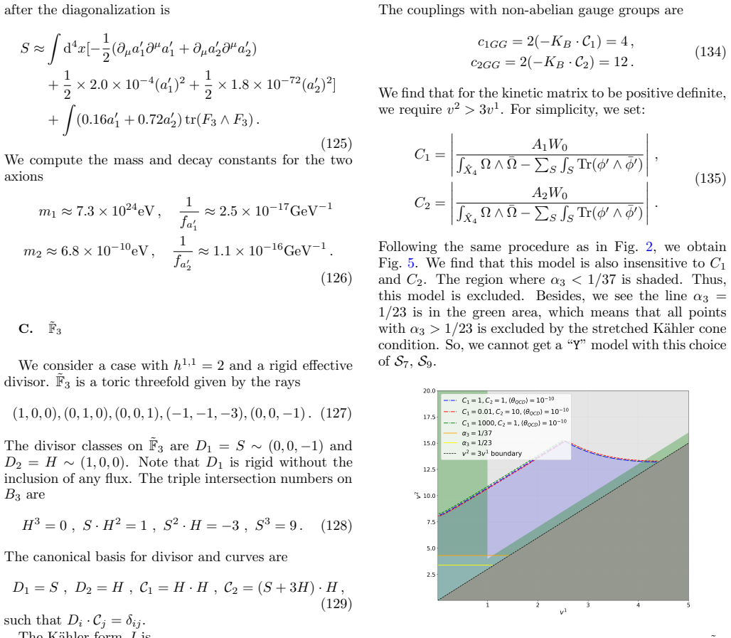
(123) We compute the mass and decay constants for the two axions m1 ≈4.0×10 26eV, 1 fa′ 1 ≈3.2×10 −17GeV−1 , m2 ≈1.4×10 −9eV, 1 fa′ 2 ≈2.2×10 −16GeV−1
tr(F3 ∧F 3). (123) We compute the mass and decay constants for the two axions m1 ≈4.0×10 26eV, 1 fa′ 1 ≈3.2×10 −17GeV−1 , m2 ≈1.4×10 −9eV, 1 fa′ 2 ≈2.2×10 −16GeV−1 . (124) One of these axions is very heavy, from the diagonaliza- tion of mass matrix. For Fig. 4, we choose (v 1, v2) = (2.5,1.2) and assume |C1 cosψ 1|=|C 2 cosψ 2|= 1. The action of two axion...
-
[5]
O”. determine the existence of this kind of model. This model is “O
tr(F3 ∧F 3). (125) We compute the mass and decay constants for the two axions m1 ≈7.3×10 24eV, 1 fa′ 1 ≈2.5×10 −17GeV−1 m2 ≈6.8×10 −10eV, 1 fa′ 2 ≈1.1×10 −16GeV−1 . (126) C. ˜F3 We consider a case withh 1,1 = 2 and a rigid effective divisor. ˜F3 is a toric threefold given by the rays (1,0,0),(0,1,0),(0,0,1),(−1,−1,−3),(0,0,−1).(127) The divisor classes on...
-
[6]
(136) The axion masses and decay constants are m1 ≈2.2×10 23eV, 1 fa′ 1 ≈7.0×10 −17GeV−1 , m2 ≈1.6×10 −9eV, 1 fa′ 2 ≈2.6×10 −16GeV−1
tr(F3 ∧F 3). (136) The axion masses and decay constants are m1 ≈2.2×10 23eV, 1 fa′ 1 ≈7.0×10 −17GeV−1 , m2 ≈1.6×10 −9eV, 1 fa′ 2 ≈2.6×10 −16GeV−1 . (137) D.P 1 ×P 1 ×P 1 This is a case withh 1,1(B) = 3 and no rigid effector divisor.P 1 ×P 1 ×P 1 is a toric threefold given by the rays (1,0,0),(0,1,0),(0,0,1),(−1,0,0),(0,−1,0),(0,0,−1). (138) The divisor cl...
-
[7]
(147) We compute the mass and decay constants of three axions m1 ≈5.8×10 12eV, 1 fa′ 1 ≈6.0×10 −17GeV−1 , m2 ≈1.4×10 −9eV, 1 fa′ 2 ≈2.3×10 −16GeV−1 , m3 ≈7.9×10 −16eV, 1 fa′ 3 = 0
tr(F3 ∧F 3). (147) We compute the mass and decay constants of three axions m1 ≈5.8×10 12eV, 1 fa′ 1 ≈6.0×10 −17GeV−1 , m2 ≈1.4×10 −9eV, 1 fa′ 2 ≈2.3×10 −16GeV−1 , m3 ≈7.9×10 −16eV, 1 fa′ 3 = 0. (148) Note thata ′ 3 does not couple to the Standard Model gauge groups. For the case of Fig. 9, we choose (v 1, v2, v2) = (1.1,1.1,1.9) and assume|C 1 cosψ 1|=|C ...
-
[8]
tr(F3 ∧F 3). (149) 16 We compute the mass and decay constants of three axions m1 ≈1.0×10 −3eV, 1 fa′ 1 ≈4.8×10 −17GeV−1 , m2 ≈7.1×10 −10eV, 1 fa′ 2 ≈1.2×10 −16GeV−1 , m3 ≈2.2×10 −27eV, 1 fa′ 3 = 0. (150) Note thata ′ 3 does not couple to the Standard Model gauge groups. V. FILTER OUT GEOMETRIC BACKGROUND As discussed previously, certain geometric back- gr...
-
[9]
This is also important to stabilize all the K¨ ahler moduli
To have a strong physical constraint on the K¨ ahler moduli space, we should assume that at least h1,1(B3) linearly independent divisors onB 3, called Dα are rigid or rigidified. This is also important to stabilize all the K¨ ahler moduli. In constrast, if the divisors are all non-rigid, noV U V arises from the string theory perspective, and the IR axion ...
-
[10]
As shown in Figs 2-6, even if we vary the Pfaffian coefficients by 3 orders of magnitude, the exclusion curves only slightly differ
The constraint on the K¨ ahler moduli space is in- sensitive to the Pfaffian coefficientsA D. As shown in Figs 2-6, even if we vary the Pfaffian coefficients by 3 orders of magnitude, the exclusion curves only slightly differ
-
[11]
N” means that no such “Y
As forf a, we estimate that the axion decay con- stantf a is generally close to the string scale in the models used in this paper. Form a, it may be sub- ject to further UV corrections, and we generally allow our string-theoretic axions to locate in the right and bottom side of the QCD axion line in Fig 1. We pinpoint the axion mass and axion de- cay cons...
-
[12]
R. D. Peccei and H. R. Quinn, CP Conservation in the Presence of Instantons, Phys. Rev. Lett.38, 1440 (1977)
1977
-
[13]
R. D. Peccei and H. R. Quinn, Constraints Imposed by CP Conservation in the Presence of Instantons, Phys. Rev. D16, 1791 (1977)
1977
-
[14]
A. E. Nelson, Naturally Weak CP Violation, Phys. Lett. B136, 387 (1984)
1984
-
[15]
R. D. Peccei, The Strong CP problem and axions, Lect. Notes Phys.741, 3 (2008), arXiv:hep-ph/0607268
work page internal anchor Pith review Pith/arXiv arXiv 2008
- [16]
-
[17]
M. Reece, TASI Lectures: (No) Global Symme- tries to Axion Physics, PoSTASI2022, 008 (2024), arXiv:2304.08512 [hep-ph]
-
[18]
Weinberg, A new light boson?, Phys
S. Weinberg, A new light boson?, Phys. Rev. Lett.40, 223 (1978)
1978
-
[19]
Wilczek, Problem of strongpandtinvariance in the presence of instantons, Phys
F. Wilczek, Problem of strongpandtinvariance in the presence of instantons, Phys. Rev. Lett.40, 279 (1978)
1978
-
[20]
Preskill, M
J. Preskill, M. B. Wise, and F. Wilczek, Cosmology of the Invisible Axion, Phys. Lett. B120, 127 (1983)
1983
-
[21]
J. E. Kim, Light Pseudoscalars, Particle Physics and Cosmology, Phys. Rept.150, 1 (1987)
1987
-
[22]
Supersymmetry, Axions and Cosmology
T. Banks, M. Dine, and M. Graesser, Supersymmetry, axions and cosmology, Phys. Rev. D68, 075011 (2003), arXiv:hep-ph/0210256
work page internal anchor Pith review Pith/arXiv arXiv 2003
-
[23]
Axions : Theory and Cosmological Role
M. Kawasaki and K. Nakayama, Axions: Theory and Cosmological Role, Ann. Rev. Nucl. Part. Sci.63, 69 (2013), arXiv:1301.1123 [hep-ph]
work page internal anchor Pith review Pith/arXiv arXiv 2013
-
[24]
D. J. E. Marsh, Axion Cosmology, Phys. Rept.643, 1 (2016), arXiv:1510.07633 [astro-ph.CO]
work page internal anchor Pith review Pith/arXiv arXiv 2016
-
[25]
I. G. Irastorza and J. Redondo, New experimental ap- proaches in the search for axion-like particles, Prog. Part. Nucl. Phys.102, 89 (2018), arXiv:1801.08127 [hep-ph]
work page internal anchor Pith review Pith/arXiv arXiv 2018
-
[26]
L. Di Luzio, M. Giannotti, E. Nardi, and L. Visinelli, The landscape of QCD axion models, Phys. Rept.870, 1 (2020), arXiv:2003.01100 [hep-ph]
- [27]
-
[28]
J. E. Kim, Weak-interaction singlet and strong CP in- variance, Phys. Rev. Lett.43, 103 (1979)
1979
-
[29]
Shifman, A
M. Shifman, A. Vainshtein, and V. Zakharov, Can con- finement ensure natural cp invariance of strong interac- tions?, Nuclear Physics B166, 493 (1980)
1980
-
[30]
M. Dine, W. Fischler, and M. Srednicki, A simple so- lution to the strong cp problem with a harmless axion, Physics Letters B104, 199 (1981)
1981
-
[31]
Zhitnitskij, On possible suppression of the axion- hadron interactions, Yad
A. Zhitnitskij, On possible suppression of the axion- hadron interactions, Yad. Fiz.31, 497–504 (1980)
1980
-
[32]
Preskill, M
J. Preskill, M. B. Wise, and F. Wilczek, Cosmology of the invisible axion, Physics Letters B120, 127 (1983)
1983
-
[33]
Abbott and P
L. Abbott and P. Sikivie, A cosmological bound on the invisible axion, Physics Letters B120, 133 (1983)
1983
-
[34]
Dine and W
M. Dine and W. Fischler, The not-so-harmless axion, Physics Letters B120, 137 (1983)
1983
-
[35]
M. I. Vysotsky, Y. B. Zeldovich, M. Y. Khlopov, and V. M. Chechetkin, Some Astrophysical Limitations on Axion Mass, Pisma Zh. Eksp. Teor. Fiz.27, 533 (1978)
1978
-
[36]
Z. G. Berezhiani and M. Y. Khlopov, Cosmology of Spontaneously Broken Gauge Family Symmetry, Z. Phys. C49, 73 (1991)
1991
-
[37]
Z. G. Berezhiani, A. S. Sakharov, and M. Y. Khlopov, Primordial background of cosmological axions, Sov. J. Nucl. Phys.55, 1063 (1992)
1992
-
[38]
M. Y. Khlopov, A. S. Sakharov, and D. D. Sokoloff, The large scale modulation of the density distribu- tion in standard axionic CDM and its cosmological and physical impact, in2nd International Workshop on Birth of the Universe and Fundamental Physics(1998) arXiv:hep-ph/9812286
work page internal anchor Pith review Pith/arXiv arXiv 1998
-
[39]
Khlopov, A
M. Khlopov, A. Sakharov, and D. Sokoloff, The non- linear modulation of the density distribution in stan- dard axionic cdm and its cosmological impact, Nuclear Physics B - Proceedings Supplements72, 105 (1999), proceedings of the 5th IFT Workshop on Axions
1999
-
[40]
Khlopov, S
M. Khlopov, S. Rubin, and A. Sakharov, Primordial structure of massive black hole clusters, Astroparticle Physics23, 265 (2005)
2005
-
[41]
Axionlimits,https://cajohare.github.io/ AxionLimits/
-
[42]
Choi and J
K. Choi and J. E. Kim, Harmful Axions in Super- string Models, Phys. Lett. B154, 393 (1985), [Erratum: Phys.Lett.B 156, 452 (1985)]
1985
-
[43]
T. Banks and M. Dine, The Cosmology of string theo- retic axions, Nucl. Phys. B505, 445 (1997), arXiv:hep- th/9608197
-
[44]
Couplings and Scales in Strongly Coupled Heterotic String Theory
T. Banks and M. Dine, Couplings and scales in strongly coupled heterotic string theory, Nucl. Phys. B479, 173 (1996), arXiv:hep-th/9605136
work page internal anchor Pith review Pith/arXiv arXiv 1996
-
[45]
J. P. Conlon, The QCD axion and moduli stabilisation, JHEP05, 078, arXiv:hep-th/0602233
work page internal anchor Pith review Pith/arXiv arXiv
-
[46]
P. Svrcek and E. Witten, Axions In String Theory, JHEP06, 051, arXiv:hep-th/0605206
work page internal anchor Pith review Pith/arXiv arXiv
-
[47]
String compactification, QCD axion and axion-photon-photon coupling
K.-S. Choi, I.-W. Kim, and J. E. Kim, String compacti- fication, QCD axion and axion-photon-photon coupling, JHEP03, 116, arXiv:hep-ph/0612107
work page internal anchor Pith review Pith/arXiv arXiv
-
[48]
T. W. Grimm, Axion inflation in type II string theory, Phys. Rev. D77, 126007 (2008), arXiv:0710.3883 [hep- th]
work page internal anchor Pith review Pith/arXiv arXiv 2008
-
[49]
Gravity Waves and Linear Inflation from Axion Monodromy
L. McAllister, E. Silverstein, and A. Westphal, Grav- ity Waves and Linear Inflation from Axion Monodromy, Phys. Rev. D82, 046003 (2010), arXiv:0808.0706 [hep- th]
work page internal anchor Pith review Pith/arXiv arXiv 2010
-
[50]
A. Arvanitaki, S. Dimopoulos, S. Dubovsky, N. Kaloper, and J. March-Russell, String Axiverse, Phys. Rev. D81, 123530 (2010), arXiv:0905.4720 [hep-th]
work page internal anchor Pith review Pith/arXiv arXiv 2010
-
[51]
Exploring the String Axiverse with Precision Black Hole Physics
A. Arvanitaki and S. Dubovsky, Exploring the String Axiverse with Precision Black Hole Physics, Phys. Rev. D83, 044026 (2011), arXiv:1004.3558 [hep-th]
work page internal anchor Pith review Pith/arXiv arXiv 2011
-
[52]
B. S. Acharya, K. Bobkov, and P. Kumar, An M Theory Solution to the Strong CP Problem and Constraints on the Axiverse, JHEP11, 105, arXiv:1004.5138 [hep-th]
work page internal anchor Pith review Pith/arXiv arXiv
-
[53]
Axions as Quintessence in String Theory
S. Panda, Y. Sumitomo, and S. P. Trivedi, Axions as Quintessence in String Theory, Phys. Rev. D83, 083506 (2011), arXiv:1011.5877 [hep-th]
work page internal anchor Pith review Pith/arXiv arXiv 2011
-
[54]
The type IIB string axiverse and its low-energy phenomenology
M. Cicoli, M. Goodsell, and A. Ringwald, The type IIB string axiverse and its low-energy phenomenology, 20 JHEP10, 146, arXiv:1206.0819 [hep-th]
work page internal anchor Pith review Pith/arXiv arXiv
-
[55]
Searching for axions and ALPs from string theory
A. Ringwald, Searching for axions and ALPs from string theory, J. Phys. Conf. Ser.485, 012013 (2014), arXiv:1209.2299 [hep-ph]
work page internal anchor Pith review Pith/arXiv arXiv 2014
-
[56]
Dark energy from the string axiverse
M. Kamionkowski, J. Pradler, and D. G. E. Walker, Dark energy from the string axiverse, Phys. Rev. Lett. 113, 251302 (2014), arXiv:1409.0549 [hep-ph]
work page internal anchor Pith review Pith/arXiv arXiv 2014
-
[57]
T. C. Bachlechner, C. Long, and L. McAllister, Planckian Axions in String Theory, JHEP12, 042, arXiv:1412.1093 [hep-th]
work page internal anchor Pith review Pith/arXiv arXiv
-
[58]
C. Long, L. McAllister, and J. Stout, Systematics of Axion Inflation in Calabi-Yau Hypersurfaces, JHEP02, 014, arXiv:1603.01259 [hep-th]
work page internal anchor Pith review Pith/arXiv arXiv
-
[59]
Cosmological window onto the string axiverse and the supersymmetry breaking scale
L. Visinelli and S. Vagnozzi, Cosmological window onto the string axiverse and the supersymmetry breaking scale, Phys. Rev. D99, 063517 (2019), arXiv:1809.06382 [hep-ph]
work page internal anchor Pith review Pith/arXiv arXiv 2019
-
[60]
M. Demirtas, C. Long, L. McAllister, and M. Still- man, The Kreuzer-Skarke Axiverse, JHEP04, 138, arXiv:1808.01282 [hep-th]
work page internal anchor Pith review Pith/arXiv arXiv
-
[61]
M. Demirtas, N. Gendler, C. Long, L. McAllister, and J. Moritz, PQ axiverse, JHEP06, 092, arXiv:2112.04503 [hep-th]
- [62]
-
[63]
N. Gendler, D. J. E. Marsh, L. McAllister, and J. Moritz, Glimmers from the axiverse, JCAP09, 071, arXiv:2309.13145 [hep-th]
-
[64]
P. Agrawal, M. Nee, and M. Reig, Axion couplings in heterotic string theory, JHEP02, 188, arXiv:2410.03820 [hep-ph]
-
[65]
V. Loladze, A. Platschorre, and M. Reig, Higher axion strings, JHEP08, 182, arXiv:2503.18707 [hep-ph]
-
[66]
J. Cheng and N. Gendler, Universality in the axiverse, JHEP11, 012, arXiv:2507.12516 [hep-th]
-
[67]
R. Petrossian-Byrne and G. Villadoro, Open string ax- iverse, JHEP07, 049, arXiv:2503.16387 [hep-ph]
- [68]
- [69]
-
[70]
M. Reig and T. Weigand, Testing the heterotic string with the axion-photon coupling, JHEP01, 006, arXiv:2509.08042 [hep-th]
-
[71]
P. Agrawal, M. Nee, and M. Reig, Axion couplings in Orbifold GUTs, arXiv (2025), arXiv:2511.21830 [hep- ph]
- [72]
-
[73]
C. Vafa, Evidence for F theory, Nucl. Phys. B469, 403 (1996), arXiv:hep-th/9602022
work page internal anchor Pith review Pith/arXiv arXiv 1996
-
[74]
D. R. Morrison and C. Vafa, Compactifications of F theory on Calabi-Yau threefolds. 1, Nucl. Phys.B473, 74 (1996), arXiv:hep-th/9602114 [hep-th]
work page internal anchor Pith review Pith/arXiv arXiv 1996
-
[75]
D. R. Morrison and C. Vafa, Compactifications of F theory on Calabi-Yau threefolds. 2., Nucl. Phys. B476, 437 (1996), arXiv:hep-th/9603161
work page internal anchor Pith review Pith/arXiv arXiv 1996
-
[76]
GUTs and Exceptional Branes in F-theory - I
C. Beasley, J. J. Heckman, and C. Vafa, GUTs and Exceptional Branes in F-theory - I, JHEP01, 058, arXiv:0802.3391 [hep-th]
work page internal anchor Pith review Pith/arXiv arXiv
-
[77]
GUTs and Exceptional Branes in F-theory - II: Experimental Predictions
C. Beasley, J. J. Heckman, and C. Vafa, GUTs and Ex- ceptional Branes in F-theory - II: Experimental Predic- tions, JHEP01, 059, arXiv:0806.0102 [hep-th]
work page internal anchor Pith review Pith/arXiv arXiv
-
[78]
R. Donagi and M. Wijnholt, Model Building with F- Theory, Adv. Theor. Math. Phys.15, 1237 (2011), arXiv:0802.2969 [hep-th]
work page internal anchor Pith review Pith/arXiv arXiv 2011
-
[79]
T. W. Grimm, The N=1 effective action of F-theory compactifications, Nucl. Phys. B845, 48 (2011), arXiv:1008.4133 [hep-th]
work page internal anchor Pith review Pith/arXiv arXiv 2011
-
[80]
The F-theory geometry with most flux vacua
W. Taylor and Y.-N. Wang, The F-theory geometry with most flux vacua, JHEP12, 164, arXiv:1511.03209 [hep-th]
work page internal anchor Pith review Pith/arXiv arXiv
discussion (0)
Sign in with ORCID, Apple, or X to comment. Anyone can read and Pith papers without signing in.