arxiv: 2605.04997 · v1 · submitted 2026-05-06 · 💻 cs.LG

Recognition: unknown

DualTCN: A Physics-Constrained Temporal Convolutional Network for 2 Time-Domain Marine CSEM Inversion

Ghada Omar, Khaled Ahmed

Authors on Pith no claims yet

Pith reviewed 2026-05-08 16:47 UTC · model grok-4.3

classification 💻 cs.LG

keywords marine CSEMtime-domain inversiontemporal convolutional networkphysics-constrained learningelectromagnetic data inversionsubsurface parameter estimationsoft-step decoderdeep learning inversion

0 comments

The pith

DualTCN regresses four earth-model parameters from marine CSEM transients and reconstructs conductivity profiles via a differentiable soft-step decoder to deliver faster and more accurate inversion than local optimization methods.

A machine-rendered reading of the paper's core claim, the machinery that carries it, and where it could break.

The paper establishes that a temporal convolutional network can invert time-domain marine controlled-source electromagnetic data by directly predicting the conductivity and thickness values of a two-layer subsurface model rather than solving a discretized inverse problem iteratively. This parameter-regression approach, followed by a physics-constrained decoder that assembles the conductivity-depth profile, produces lower error on synthetic test cases while running orders of magnitude faster than conventional solvers. A sympathetic reader would care because traditional inversion of such data has historically required heavy computation and repeated forward modeling, limiting its use in large surveys or time-sensitive applications. The work also shows that targeted data augmentation makes the network robust to realistic amplitude noise and that the same structure extends reasonably to three-layer models.

Core claim

DualTCN is a deep-learning framework that inverts time-domain marine CSEM transients by regressing the four parameters σ1, σ2, d1, d2 of a layered earth model and then reconstructing the conductivity-depth profile with a differentiable soft-step decoder; the optimized TCN encoder with late-time branch and auxiliary seafloor-depth head yields a 25.3 percent loss reduction over baselines, mean R-squared of 0.877, and up to 21,000-fold reduction in compute time relative to Levenberg-Marquardt or L-BFGS-B while remaining robust to noise through curriculum amplitude augmentation.

What carries the argument

DualTCN architecture: a Temporal Convolutional Network encoder paired with a late-time branch, an auxiliary seafloor-depth head, and a differentiable soft-step decoder that converts the four regressed parameters into a conductivity-depth profile.

If this is right

Inversion speed reaches 3.5 milliseconds per sample on an A100 GPU, making large-scale or repeated inversions practical.
Mean predictive accuracy across the four parameters reaches R-squared of 0.877, with the strongest result on the second-layer conductivity.
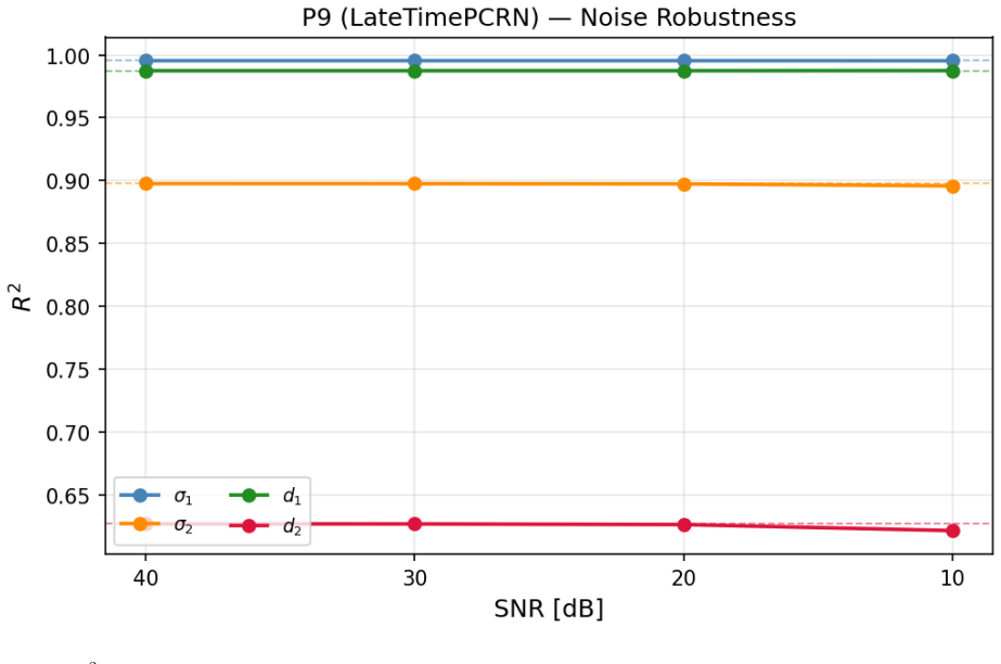
Curriculum-based amplitude augmentation raises noise robustness so that mean R-squared remains 0.858 even at plus or minus 2 percent random error.
Monte Carlo dropout supplies uncertainty estimates that are well-calibrated for shallow conductivity but require post-hoc scaling for deeper thickness.
The same network structure generalizes to three-layer models and recovers basement conductivity with R-squared approximately 0.88.

Where Pith is reading between the lines

These are editorial extensions of the paper, not claims the author makes directly.

The parameter-regression-plus-decoder pattern could be adapted to other electromagnetic or potential-field inversion tasks that currently rely on iterative local optimization.
Real-time marine survey interpretation becomes feasible if the network is embedded in acquisition hardware or shipboard processing pipelines.
The thin-layer resolution limit (R-squared approximately 0.23) indicates that multi-offset or multi-frequency data would be needed to extend the method beyond simple layered cases.
Hybrid workflows that use the fast DualTCN output as a starting model for a final physics-based refinement step could combine speed with higher fidelity on complex geology.

Load-bearing premise

The true subsurface can be adequately represented by a two-layer model whose conductivity and thickness parameters are recovered accurately enough that the soft-step decoder produces profiles whose forward responses match the input data within noise levels at the offsets used.

What would settle it

Generate synthetic CSEM transients from a known three-dimensional or finely layered conductivity model, run DualTCN inversion, then forward-model the recovered two-layer parameters and observe whether the mismatch between predicted and input data exceeds the level attributable to added noise.

Figures

Figures reproduced from arXiv: 2605.04997 by Ghada Omar, Khaled Ahmed.

**Figure 1.** Figure 1: (a) MCSEM acquisition geometry. The HED source sits at depth view at source ↗

**Figure 2.** Figure 2: Architecture of DualTCN (379 000 parameters). view at source ↗

**Figure 3.** Figure 3: DualTCN predictions on six test samples. Left: normalised E-field traces from four receivers. Right: true profile view at source ↗

**Figure 4.** Figure 4: Absolute d2 prediction error (normalised) versus true d2 (5 000 test samples), coloured by σ1/σ2. Errors are largest for thin layers with weak contrast (upper-left). 25 view at source ↗

**Figure 5.** Figure 5: R2 versus SNR for DualTCN (150 000 test samples). All parameters maintain clean-test values above 20 dB; at 10 dB the worst decline is ∆R2 = 0.005 (d2) view at source ↗

**Figure 6.** Figure 6: True versus predicted scatter for DualTCN (5 000 test samples, normalised view at source ↗

**Figure 7.** Figure 7: DualTCN R2 as a function of amplitude-channel perturbation strength (150 000 test samples). Panel (A): random noise σamp in log10 units (top axis: approximate amplitude uncertainty %). Panel (B): systematic bias β in log10 units (top axis: multiplicative amplitude factor 10β). In both panels, σ2 (orange) and d2 (red) degrade rapidly because they rely primarily on the log-amplitude channel, while d1 (green)… view at source ↗

**Figure 8.** Figure 8: Amplitude robustness of Base, AmpAug, and AmpRatio variants under structured perturbations (150 000 test samples). view at source ↗

read the original abstract

DualTCN is the first deep-learning framework for inverting time-domain marine controlled-source electromagnetic (MCSEM) transient data. Moving away from traditional subsurface discretization, the framework regresses four earth-model parameters -- $\sigma_1$, $\sigma_2$, $d_1$, $d_2$ -- and reconstructs conductivity-depth profiles using a differentiable soft-step decoder. The optimized architecture (379K parameters) features a Temporal Convolutional Network (TCN) encoder paired with a late-time branch and an auxiliary seafloor-depth head. This design achieves a 25.3\% loss reduction over baseline models, with high predictive accuracy ($R^2 = 0.898$ for $\sigma_2$) and an inversion speed of 3.5~ms per sample on an A100 GPU. The framework demonstrates high robustness to noise through curriculum-based amplitude augmentation, maintaining a mean $\bar{R}^2$ of 0.858 at $\pm2\%$ random amplitude error, compared to $0.363$ without augmentation. DualTCN generalizes effectively to three-layer extensions (seawater/resistive layer/basement), accurately resolving basement conductivity ($R^2 \approx 0.88$), though thin-layer resolution remains a physical limitation ($R^2 \approx 0.23$). In comparative benchmarks, DualTCN significantly outperforms traditional local optimization methods like Levenberg-Marquardt and L-BFGS-B, yielding a mean $\bar{R}^2 = 0.877$ versus 0.129-0.439 for multi-start baselines, while operating at up to 21,000$\times$ lower computational cost. Finally, the framework incorporates uncertainty quantification via Monte Carlo (MC) Dropout. While well-calibrated for $\sigma_1$ (PICP90 = 0.944), inherent signal limitations at short offsets (200m) lead to under-coverage for $d_2$ (PICP90 = 0.572), which can be mitigated through post-hoc temperature scaling or split conformal prediction.

Editorial analysis

A structured set of objections, weighed in public.

Desk editor's note, referee report, simulated authors' rebuttal, and a circularity audit. Tearing a paper down is the easy half of reading it; the pith above is the substance, this is the friction.

Desk Editor's Note private letter to a colleague

DualTCN regresses four parameters from time-domain MCSEM transients with a TCN and soft-step decoder for speed on two-layer synthetics, but the decoder approximation and narrow model scope are the points to verify.

read the letter

DualTCN regresses four earth parameters from time-domain marine CSEM transients using a TCN encoder, then reconstructs the conductivity profile with a differentiable soft-step decoder. It reports a 25% loss improvement over baselines, R² near 0.9 for conductivity, and up to 21,000 times faster runtime than Levenberg-Marquardt on an A100, plus noise robustness from curriculum augmentation and MC dropout uncertainty estimates. The late-time branch and auxiliary seafloor head are the main architectural additions. The three-layer generalization test is a reasonable check even if thin layers stay difficult. The soft-step decoder is a clean way to stay physics-constrained without full discretization. The numbers are concrete and the speed claim is the clearest practical win. The two-layer assumption is a real limit for field data, and the stress-test point on decoder smoothing at 200 m offsets looks worth checking against the forward model; any mismatch there could make the R² figures optimistic. The low PICP for the deeper depth parameter is also a practical drawback. Training data generation and split details would help confirm the test set is independent. This is for marine geophysicists who already run MCSEM surveys and want faster synthetic inversions, or for ML people working on physics-informed networks for EM. It has enough specific claims and comparisons to go to a serious referee rather than a desk reject. Send it out, with the expectation that reviewers will focus on decoder fidelity and how far the simple model can stretch.

Referee Report

2 major / 3 minor

Summary. The manuscript introduces DualTCN, the first deep-learning framework for inverting time-domain marine controlled-source electromagnetic (MCSEM) transient data. It regresses four earth-model parameters (σ₁, σ₂, d₁, d₂) from TCN-encoded transients and reconstructs conductivity-depth profiles via a differentiable soft-step decoder, augmented by a late-time branch and auxiliary seafloor-depth head. The 379K-parameter model reports a 25.3% loss reduction over baselines, R²=0.898 for σ₂, mean R²=0.877, 3.5 ms inference (up to 21,000× faster than Levenberg-Marquardt or L-BFGS-B), noise robustness via curriculum amplitude augmentation (mean R²=0.858 at ±2% error), generalization to three-layer models (basement R²≈0.88), and uncertainty quantification via MC Dropout (PICP90=0.944 for σ₁ but 0.572 for d₂).

Significance. If the central claims hold after addressing decoder fidelity, this would be a significant contribution to physics-constrained ML for geophysical inversion. The explicit speed-accuracy tradeoff versus local optimization methods, combined with curriculum training for robustness and MC-Dropout uncertainty, addresses practical bottlenecks in marine CSEM workflows. The differentiable decoder approach to enforcing two-layer (and extensible three-layer) physics without full discretization is a clear strength that could generalize to other transient EM problems.

major comments (2)

[Methods (differentiable soft-step decoder)] Methods (differentiable soft-step decoder description): The headline metrics (25.3% loss reduction, R²=0.898 for σ₂, mean R²=0.877) rest on the decoder accurately mapping regressed parameters to conductivity profiles whose forward responses match the data-generating two-layer model to within the 2% noise level. At the 200 m offsets used, late-time transients are sensitive to interface location and sharpness; no quantitative bound on decoder approximation error (e.g., L2 mismatch in reconstructed vs. true forward responses or sensitivity to transition width) is supplied. This must be added, as any systematic mismatch would render the reported accuracy and robustness figures optimistic.
[Results (three-layer generalization)] Results (three-layer extension and thin-layer resolution): The claim that thin-layer R²≈0.23 is purely a physical limitation (rather than decoder-induced) requires an ablation that compares the soft-step decoder against direct parameter regression or a hard-step baseline on the same short-offset data. Without this, it remains unclear whether the reported basement conductivity accuracy (R²≈0.88) generalizes reliably or is inflated by the two-layer training distribution.

minor comments (3)

[Abstract and Results] Abstract and §4: The PICP90=0.572 for d₂ is correctly flagged as under-coverage due to short-offset signal limits; the post-hoc mitigation via temperature scaling or split conformal prediction should be shown with before/after calibration plots for all four parameters.
[Experimental setup] Experimental details: Full specification of data-generation procedure (including exact offset ranges, time windows, and how the 2% amplitude noise is sampled during curriculum training) and train/validation/test splits is required for reproducibility of the 25.3% loss reduction.
[Architecture] Notation: The auxiliary seafloor-depth head is mentioned but its loss weighting relative to the main parameter regression loss is not stated; clarify in the architecture diagram or equations.

Simulated Author's Rebuttal

2 responses · 0 unresolved

We thank the referee for the constructive and detailed comments on our manuscript introducing DualTCN for time-domain marine CSEM inversion. The feedback highlights important aspects of decoder fidelity and generalization that we will address to strengthen the paper. Below we provide point-by-point responses to the major comments.

read point-by-point responses

Referee: Methods (differentiable soft-step decoder description): The headline metrics (25.3% loss reduction, R²=0.898 for σ₂, mean R²=0.877) rest on the decoder accurately mapping regressed parameters to conductivity profiles whose forward responses match the data-generating two-layer model to within the 2% noise level. At the 200 m offsets used, late-time transients are sensitive to interface location and sharpness; no quantitative bound on decoder approximation error (e.g., L2 mismatch in reconstructed vs. true forward responses or sensitivity to transition width) is supplied. This must be added, as any systematic mismatch would render the reported accuracy and robustness figures optimistic.

Authors: We agree that an explicit quantitative bound on the soft-step decoder's approximation error is necessary to support the headline metrics and ensure they are not optimistic. In the revised manuscript, we will add to the Methods section a dedicated analysis that computes the L2 mismatch between forward-modeled responses of the decoded conductivity profiles and the ground-truth two-layer models, along with a sensitivity study varying the transition width parameter. This will confirm that the decoder error remains below the 2% noise level used in training and evaluation. revision: yes
Referee: Results (three-layer extension and thin-layer resolution): The claim that thin-layer R²≈0.23 is purely a physical limitation (rather than decoder-induced) requires an ablation that compares the soft-step decoder against direct parameter regression or a hard-step baseline on the same short-offset data. Without this, it remains unclear whether the reported basement conductivity accuracy (R²≈0.88) generalizes reliably or is inflated by the two-layer training distribution.

Authors: We acknowledge that an ablation is required to rigorously separate physical limitations from potential decoder effects in the three-layer generalization results. We will add this ablation to the revised Results section, comparing the soft-step decoder against (i) direct regression of the four parameters without any decoder and (ii) a hard-step (discontinuous) baseline, all evaluated on the same short-offset three-layer test data. The outcomes will be used to substantiate that the thin-layer R²≈0.23 reflects a physical resolution limit at 200 m offsets rather than decoder bias, while the basement conductivity R²≈0.88 remains reliable. revision: yes

Circularity Check

0 steps flagged

Derivation chain is self-contained; no load-bearing steps reduce to inputs by construction

full rationale

The framework regresses four parameters (σ1, σ2, d1, d2) via a TCN encoder and reconstructs profiles with a differentiable soft-step decoder; reported metrics (R²=0.898 for σ2, 25.3% loss reduction, mean R²=0.877) are computed on held-out test data after supervised training, not by equating outputs to fitted inputs. The physics constraint is architectural (decoder enforces two-layer structure) rather than definitional. No self-citations, uniqueness theorems, or ansatzes are invoked to force the central claims; curriculum augmentation and MC dropout are standard techniques evaluated externally. The derivation therefore remains independent of its own fitted values.

Axiom & Free-Parameter Ledger

1 free parameters · 2 axioms · 2 invented entities

The central claim rests on a two-layer earth model assumption and the effectiveness of a custom differentiable decoder; the network weights are learned from data.

free parameters (1)

TCN network weights and hyperparameters
379K parameters are fitted during training to map transient signals to the four earth parameters.

axioms (2)

domain assumption Subsurface conductivity structure can be represented by two layers with parameters σ1, σ2, d1, d2
The regression targets and soft-step reconstruction assume this simple layered model suffices.
domain assumption The soft-step decoder produces a sufficiently accurate continuous conductivity profile
Used to make the model physics-constrained and differentiable.

invented entities (2)

Differentiable soft-step decoder no independent evidence
purpose: Convert four discrete layer parameters into a smooth conductivity-depth profile for end-to-end training
Custom component introduced to incorporate physics constraints.
Late-time branch no independent evidence
purpose: Capture late-time signal behavior within the TCN encoder
Part of the optimized architecture described.

pith-pipeline@v0.9.0 · 5692 in / 1739 out tokens · 65248 ms · 2026-05-08T16:47:50.748010+00:00 · methodology

discussion (0)

Reference graph

Works this paper leans on

27 extracted references · 27 canonical work pages

[1]

Inverse Problems 28, 123012

Inversion algorithms for large-scale geophysical electromagnetic measurements. Inverse Problems 28, 123012. doi:10.1088/0266-5611/28/12/123012. Angelopoulos, A.N., Bates, S.,

work page doi:10.1088/0266-5611/28/12/123012
[2]

and Bates, Stephen , title =

Conformal prediction: A gentle introduction. Foundations and Trends in Machine Learning 16, 494–591. doi:10.1561/2200000101. 20 Araya-Polo, M., Jennings, J., Adler, A., Dahlke, T.,

work page doi:10.1561/2200000101
[3]

The Leading Edge 37, 58–66

Deep-learning tomography. The Leading Edge 37, 58–66. doi:10.1190/tle37010058.1. Ardizzone, L., Kruse, J., Wirkert, S., Rahner, D., Pellegrini, E.W., Klessen, R.S., Maier-Hein, L., Rother, C., Köthe, U.,

work page doi:10.1190/tle37010058.1
[4]

Analyzing inverse problems with invertible neural networks, in: Proc. Int. Conf. Learn. Represent. (ICLR). [Online]. Available:https://arxiv.org/abs/1808.04730. Bai, P., Vignoli, G., Hansen, T.M.,

work page arXiv
[5]

Geophysical Journal International 237, 1–15

Unsupervised deep learning magnetotelluric inversion. Geophysical Journal International 237, 1–15. doi:10.1093/gji/ggae005. Byrd, R.H., Lu, P., Nocedal, J., Zhu, C.,

work page doi:10.1093/gji/ggae005
[6]

A limited memory algorithm for bound constrained optimization. SIAM J. Sci. Comput. 16, 1190–1208. doi:10.1137/0916069. Colombo, D., Turkoglu, E., Li, W., Sandoval-Curiel, E., Rovetta, D.,

work page doi:10.1137/0916069
[7]

Geophysics 86, B225–B245

Physics-driven deep learning electromagnetic data inversion with applications to subsurface imaging. Geophysics 86, B225–B245. doi:10.1190/geo2020-0759.1. Constable, S.,

work page doi:10.1190/geo2020-0759.1
[8]

Geophysics 75, 75A67–75A81

Ten years of marine CSEM for hydrocarbon exploration. Geophysics 75, 75A67–75A81. doi:10.1190/1.3483451. Constable, S., Srnka, L.J.,

work page doi:10.1190/1.3483451
[9]

Geophysics 72, WA3–WA12

An introduction to marine controlled-source electromagnetic methods for hydrocarbon exploration. Geophysics 72, WA3–WA12. doi:10.1190/1.2432483. Constable, S.C., Parker, R.L., Constable, C.G.,

work page doi:10.1190/1.2432483
[10]

Geophysics 52, 289–300

Occam’s inversion: A practical algorithm for generating smooth models from electromagnetic sounding data. Geophysics 52, 289–300. doi:10.1190/1.1442303. Gal, Y., Ghahramani, Z.,

work page doi:10.1190/1.1442303
[11]

A., Law, K

Ensemble Kalman methods for inverse problems. Inverse Problems 29, 045001. doi:10.1088/0266-5611/29/4/045001. Key, K.,

work page doi:10.1088/0266-5611/29/4/045001
[12]

Geophysics 74, F9–F20

1D inversion of multicomponent, multifrequency marine CSEM data: Methodology and synthetic studies for resolving thin resistive layers. Geophysics 74, F9–F20. doi:10.1190/1.3058434. Key, K.,

work page doi:10.1190/1.3058434
[13]

Surveys in Geophysics 33, 135–167

Marine electromagnetic studies of seafloor resources and tectonics. Surveys in Geophysics 33, 135–167. doi:10.1007/s10712-011-9139-x. 21 Lakshminarayanan, B., Pritzel, A., Blundell, C.,

work page doi:10.1007/s10712-011-9139-x
[14]

Simple and Scalable Predictive Uncertainty Estimation using Deep Ensembles

Simple and scalable predictive uncertainty estimation using deep ensembles, in: Advances in Neural Information Processing Systems (NeurIPS), pp. 6402–6413. [Online]. Available:https://arxiv.org/abs/1612.01474. LeCun, Y., Bengio, Y., Hinton, G.,

work page Pith review arXiv
[15]

LeCun, Y

Deep learning. Nature 521, 436–444. doi:10.1038/nature14539. Li, G., et al.,

work page doi:10.1038/nature14539
[16]

Geophysical Prospecting doi:10.1111/1365-2478.13622

One-dimensional deep learning inversion of marine controlled-source electromagnetic data. Geophysical Prospecting doi:10.1111/1365-2478.13622. early access. Liu, W., Wang, H., Xi, Z., Zhou, L.,

work page doi:10.1111/1365-2478.13622
[17]

IEEE Trans

Physics-driven deep learning inversion with application to transient electromagnetic data. IEEE Trans. Geosci. Remote Sens. 60, 5901212. doi:10.1109/TGRS.2021.3120138. Moghadas, D.,

work page doi:10.1109/tgrs.2021.3120138 2021
[18]

Near Surface Geophysics 18, 11–32

One-dimensional deep learning inversion of electromagnetic induction data using convolutional neural network. Near Surface Geophysics 18, 11–32. doi:10.1002/nsg.12030. Moré, J.J.,

work page doi:10.1002/nsg.12030
[19]

Springer

The Levenberg–Marquardt algorithm: Implementation and theory, in: Numerical Analysis. Springer. volume 630 ofLecture Notes in Mathematics, pp. 105–116. doi:10.1007/BFb0067700. Papamakarios, G., Nalisnick, E., Rezende, D.J., Mohamed, S., Lakshminarayanan, B.,

work page doi:10.1007/bfb0067700
[20]

Geophysical Journal International 218, 817–832

Deep learning electromagnetic inversion with convolutional neural networks. Geophysical Journal International 218, 817–832. doi:10.1093/gji/ggz204. Puzyrev, V., Swidinsky, A.,

work page doi:10.1093/gji/ggz204
[21]

Computers & Geosciences 149, 104681

Inversion of 1D frequency- and time-domain electromagnetic data with convolutional neural networks. Computers & Geosciences 149, 104681. doi:10.1016/j.cageo.2020.104681. Raissi, M., Perdikaris, P., Karniadakis, G.E.,

work page doi:10.1016/j.cageo.2020.104681 2020
[22]

Physics-informed neural networks: A deep learning framework for solving forward and inverse problems involving nonlinear partial differential equations. J. Comput. Phys. 378, 686–707. doi:10.1016/j.jcp.2018.10.045. Reichstein, M., Camps-Valls, G., Stevens, B., Jung, M., Denzler, J., Carvalhais, N., Prabhat,

work page doi:10.1016/j.jcp.2018.10.045 2018
[23]

Geophysical Journal International 235, 2231–2247

Deep image prior for magnetotelluric inversion. Geophysical Journal International 235, 2231–2247. doi:10.1093/gji/ggad345. Werthmüller, D.,

work page doi:10.1093/gji/ggad345
[24]

Geophysics 82, WB9–WB19

An open-source full 3D electromagnetic modeler for 1D VTI media in Python: empymod. Geophysics 82, WB9–WB19. doi:10.1190/geo2016-0626.1. 22 Zhang, Z., Hu, Z.,

work page doi:10.1190/geo2016-0626.1
[25]

Physics-driven deep-learning for marine CSEM data inversion. J. Appl. Geophys. 229, 105497. doi:10.1016/j.jappgeo.2024.105497. Zhang, Z., Huang, J., Wan, L.,

work page doi:10.1016/j.jappgeo.2024.105497 2024
[26]

Geophysics 89, E55–E68

3-D CSEM data inversion using deep convolutional neural networks: A feasibility study. Geophysics 89, E55–E68. doi:10.1190/geo2023-0201.1. Zhu, C., Byrd, R.H., Lu, P., Nocedal, J.,

work page doi:10.1190/geo2023-0201.1
[27]

ACM Trans

Algorithm 778: L-BFGS-B: Fortran subroutines for large-scale bound-constrained optimization. ACM Trans. Math. Softw. 23, 550–560. doi:10.1145/279232.279236. 23 Figure 3: DualTCN predictions on six test samples. Left: normalised E-field traces from four receivers. Right: true profile (blue) and prediction (red dashed). 24 Figure 4: Absolute d2 prediction e...

work page doi:10.1145/279232.279236