Recognition: unknown
Nonequilibrium Fluctuation-Response Theory in the Frequency Domain
Pith reviewed 2026-05-08 16:18 UTC · model grok-4.3
The pith
The power spectrum of observables in nonequilibrium steady states equals a quadratic form of local responses at the same frequency.
A machine-rendered reading of the paper's core claim, the machinery that carries it, and where it could break.
Core claim
For systems in nonequilibrium steady states governed by overdamped Langevin dynamics or Markov jump processes, the power spectrum of a general observable is expressed exactly as a quadratic form of the local responses measured at the same frequency; the decomposition is spatial for Langevin systems and edge-resolved for jump processes.
What carries the argument
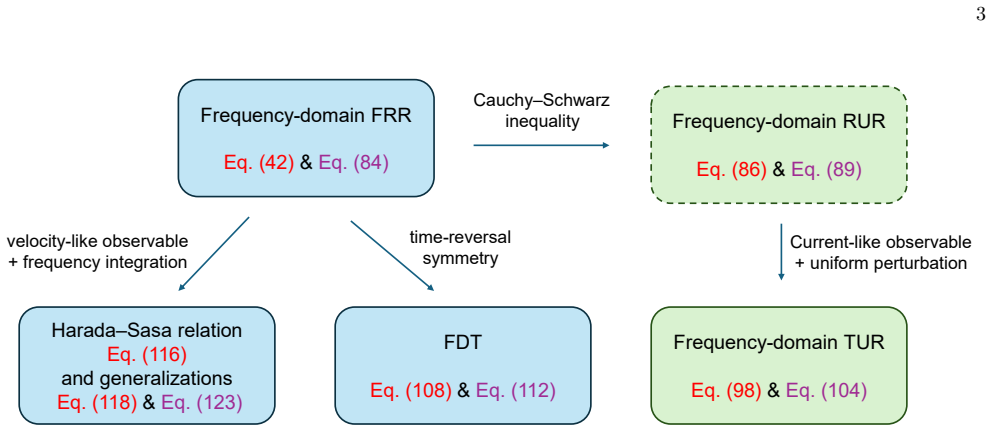
The frequency-domain fluctuation-response identity, which decomposes the power spectrum into a quadratic form of frequency-matched local responses.
If this is right
- Response uncertainty relations hold at each frequency separately.
- Kinetic and thermodynamic uncertainty relations follow directly from the same identity.
- The equilibrium fluctuation-dissipation theorem is recovered as a special case.
- Harada-Sasa-type relations appear as immediate corollaries.
- Fluctuation spectra in stochastic networks or driven diffusive systems resolve into explicit edge-wise or spatial contributions.
Where Pith is reading between the lines
- The relation suggests that frequency-dependent trade-offs between fluctuations, response speed, and dissipation can be read directly from measurable spectra without full knowledge of the underlying rates or forces.
- It may allow experimental estimation of hidden dissipation rates in biological or colloidal systems by combining fluctuation spectra with local response measurements at selected frequencies.
- Similar decompositions, if they exist, could extend the framework to underdamped or non-Markovian dynamics.
Load-bearing premise
The systems must obey overdamped Langevin dynamics or Markov jump processes and sit in a nonequilibrium steady state.
What would settle it
A direct measurement, in an overdamped Langevin or Markov-jump system, showing that the observed power spectrum at a chosen frequency deviates from the quadratic combination of the independently measured local responses at that same frequency.
Figures


read the original abstract
We develop a unified fluctuation-response theory in the frequency domain for nonequilibrium steady states governed by overdamped Langevin dynamics and Markov jump processes. The relation expresses the power spectrum of general observables exactly as a quadratic form of local responses measured at the same frequency, thereby extending static nonequilibrium fluctuation-response relations to finite frequencies. The decomposition is spatial for Langevin systems and edge-resolved for Markov jump processes, and applies uniformly to state-dependent observables, current-like observables, and their combinations. As consequences of the same identity, we derive frequency-domain response uncertainty relations, kinetic and thermodynamic uncertainty relations, the equilibrium fluctuation-dissipation theorem, and Harada-Sasa-type relations. Applications to stochastic networks and driven diffusive systems illustrate how the theory resolves fluctuation spectra into edge-wise contributions and reveals frequency-dependent tradeoffs between fluctuations, response, and dissipation.
Editorial analysis
A structured set of objections, weighed in public.
Referee Report
Summary. The manuscript develops a unified fluctuation-response theory in the frequency domain for nonequilibrium steady states (NESS) governed by overdamped Langevin dynamics and Markov jump processes. The central claim is an exact identity expressing the power spectrum of general observables (state-dependent, current-like, or combinations) as a quadratic form of local responses measured at the same frequency. This extends static nonequilibrium fluctuation-response relations to finite frequencies, with a spatial decomposition for Langevin systems and an edge-resolved decomposition for jump processes. Consequences include derivations of frequency-domain response uncertainty relations, kinetic and thermodynamic uncertainty relations, recovery of the equilibrium fluctuation-dissipation theorem, and Harada-Sasa relations. Applications to stochastic networks and driven diffusive systems illustrate resolution of fluctuation spectra into local contributions.
Significance. If the central identity holds, the work provides a significant exact framework for frequency-domain analysis in nonequilibrium stochastic thermodynamics without additional approximations for the stated dynamical classes. The uniform treatment of different observable types and the local decompositions enable new insights into how specific edges or spatial regions contribute to global spectra and frequency-dependent tradeoffs between fluctuations, response, and dissipation. Recovery of known equilibrium and nonequilibrium limits serves as a strong internal consistency check, and the derived uncertainty relations may find applications in analyzing biological and driven systems.
minor comments (3)
- [§3.2] §3.2, Eq. (18): the definition of the local response operator could include an explicit statement of its action on the probability current to clarify the edge-resolved decomposition for Markov processes.
- [Figure 2] Figure 2: the color scale for the edge contributions in the driven diffusive system example is not labeled with units, making quantitative comparison to the total spectrum difficult.
- [Introduction] The abstract states the relation is 'exact' for the two dynamical classes; a brief remark in the introduction on why the derivation does not extend immediately to underdamped Langevin dynamics would help scope the result.
Simulated Author's Rebuttal
We thank the referee for the positive and accurate summary of our manuscript on the frequency-domain fluctuation-response theory for nonequilibrium steady states. We appreciate the recognition of the exact identity's scope, its uniform treatment of observables, the local decompositions, and the recovery of known limits as consistency checks. Since the report lists no specific major comments, we have no revisions to propose at this time but remain available to address any minor points the editor or referee may identify.
Circularity Check
No significant circularity; derivation follows directly from stochastic generator
full rationale
The central identity expresses the power spectrum exactly as a quadratic form in same-frequency local responses, obtained by direct algebraic manipulation of the Fokker-Planck or master-equation generator for overdamped Langevin dynamics and Markov jump processes in NESS. No step reduces a fitted parameter to a prediction, renames a known result as new unification, or relies on a load-bearing self-citation whose content is itself unverified. Recovery of the equilibrium FDT and Harada-Sasa relations functions only as an internal consistency check. The derivation remains self-contained against the stated dynamical assumptions and does not import uniqueness theorems or ansatzes from prior author work.
Axiom & Free-Parameter Ledger
Reference graph
Works this paper leans on
-
[1]
Perturbed Fokker–Planck generator and local response formulas In this subsection, we derive the local response for- mulas stated in Sec. III. We consider the overdamped Langevin dynamics ˙x(t) =M(x(t))F(x(t)) + √ 2B(x(t))⊛ξ(t),(A1) where⊛denotes the anti-Itˆ o product, and ˆLx is the Fokker–Planck generator given by ˆLx =−∇ T x ˆJx, ˆJx =M(x) F(x)−T(x)∇ x...
-
[2]
Properties of the excess propagator In this subsection, we derive the identities for the ex- cess propagator used in Sec. III. We recall its definition, H(x,z;ω) = Z ∞ 0 P(x, t|z,0)−π(x) eiωt dt.(A24) The propagator satisfies both the forward and backward Fokker–Planck equations, ∂tP(x, t|z,0) = ˆLxP(x, t|z,0),(A25) ∂tP(x, t|z,0) = ˆL† zP(x, t|z,0),(A26) ...
-
[3]
Covariances of empirical density and current We now derive the covariance formulas for the empiri- cal density and current. We begin with ρ(x, t) =δ(x−x(t)).(A34) Fort >0, the connected two-time correlation is given by ⟨ρ(x, t)ρ(y,0)⟩ −π(x)π(y) = P(x, t|y,0)−π(x) π(y), (A35) whereas fort <0, ⟨ρ(x, t)ρ(y,0)⟩ −π(x)π(y) = P(y,−t|x,0)−π(y) π(x), (A36) which f...
-
[4]
Proof of the quadratic representation for the density–density covariance In this subsection, we prove the quadratic representa- tion (A38) of the density–density covariance. We first rewriteH(x,y;ω)π(y) in terms of a delta function to exploit the resolvent identity: H(x,y;ω)π(y) = Z dzπ(z)H(x,z;ω)δ(y−z).(A50) Using the identity (A33) we rewrite the delta ...
-
[5]
Explicit forms of the perturbation weight matricesA ϕ(z) In this subsection, we collect the explicit forms of the perturbation weight matricesA ϕ(z) that enter the FRR. We recall the definition Aϕ(z) = 1 2π(z) N ϕ(z) T D(z) −1N ϕ(z).(A55) For perturbationsϕ∈ {F,lnM, T}, using (A20)–(A22), we obtain the following explicit forms ofA ϕ(z): [AF (z)]kl =δ kl π...
-
[6]
Perturbed master equation and local response formulas In this subsection, we derive the local response for- mulas stated in Sec. IV. The structure closely parallels Appendix A 1. We consider a local perturbation applied at timet= 0 on the edgek↔l(withk > l). The unperturbed dynamics is governed by ∂tp(t) =Wp(t),(B1) with stationary distributionπsatisfying...
-
[7]
Properties of the discrete excess propagator We now derive several identities for the discrete excess propagator defined in (B15). To this end, we use the following limiting behaviors: lim t→0+ [eWt]nk =δ nk,lim t→∞ [eWt]nk =π n.(B28) First, we show that X m Hnm(ω)πm = 0.(B29) Multiplying (B15) byπ m and summing overm, we obtain X m Hnm(ω)πm = Z ∞ 0 dt ei...
-
[8]
Covariances of empirical state indicators and edge currents We now derive the covariance formulas for the empir- ical state indicators and empirical edge currents. We begin with ηn(t) =δ X(t),n .(B37) 24 Fort >0, ⟨ηn(t)ηm(0)⟩ −π nπm = [eWt]nm −π n πm,(B38) whereas fort <0, by time-translation invariance, ⟨ηn(t)ηm(0)⟩ −π nπm = [eW(−t)]mn −π m πn.(B39) Taki...
-
[9]
Proof of the discrete quadratic identity for the state–state covariance In this subsection, we prove the quadratic representa- tion (B41). To this end, we first rewriteH nm(ω)πm in terms of a Kronecker-delta function as Hnm(ω)πm = X k Hnk(ω)πkδkm.(B55) Using the identity (B36) at frequency−ω, we rewrite the Kronecker-delta as δkm =− X l −iωδlk +W lk Hml(−...
-
[10]
Derivation of the frequency-domain response uncertainty relation In this subsection, we derive the frequency-domain RUR stated in Sec. V A. This follows directly from the Cauchy–Schwarz inequality applied to the quadratic re- sponse representation of the covariance matrix. We begin with the overdamped Langevin case. For an arbitrary vectoru∈C NO, multiply...
-
[11]
We begin with the overdamped Langevin case
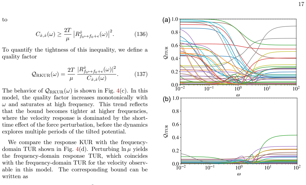
Derivation of the frequency-domain thermodynamic uncertainty relations In this subsection, we derive the frequency-domain TURs, (97) and (105). We begin with the overdamped Langevin case. Con- sider the homogeneous perturbationψ k(x, ω) = 1 (for all k,x, andω). For a current-like observable θ(t) = Z dxL(x)ȷ(x, t),(C18) the corresponding global response is...
-
[12]
Hence, for this choice of perturbation, the response equals the mean value of the current-like observable: Rθ B7→B+ϵ(ω) =⟨θ⟩ ss. This relation extends componen- twise to a vector of current-like observables Rθ B7→B+ϵ(ω) =⟨θ⟩ ss.(C26) Substituting this into (104) yields ⟨θ⟩T ssCθ,θ T(ω)−1⟨θ⟩ss ≤ σps 2 ,(C27) which is the frequency-domain TUR for Markov jum...
-
[13]
Proof of the equilibrium reciprocity identities In this subsection, we prove the reciprocity identities used in Sec. V C. We consider the overdamped Langevin and Markov jump cases separately. We begin with the overdamped Langevin case. At equilibrium, we assume spatially homogeneous temper- atureT k(x) =Tand conservative forceF k(x) = −∂xk U(x), so that t...
-
[14]
V C and V D
Alternative covariance–response identities In this subsection, we derive the alternative covariance–response identities (108) and (111) used in Secs. V C and V D. For overdamped Langevin systems, (A18) and (A20) yield the force-response formula Rȷ(x) F(y) (ω) =P(x,y;ω)M(y)π(y).(C45) Recalling the relationD(y) =M(y)T(y), we can rewrite the current-current ...
-
[15]
Kubo, Reports on Progress in Physics29, 255 (1966)
R. Kubo, Reports on Progress in Physics29, 255 (1966)
1966
-
[16]
G. S. Agarwal, Zeitschrift f¨ ur Physik A Hadrons and nu- clei252, 25 (1972)
1972
-
[17]
Speck and U
T. Speck and U. Seifert, Europhysics Letters74, 391 (2006)
2006
-
[18]
Baiesi, C
M. Baiesi, C. Maes, and B. Wynants, Phys. Rev. Lett. 103, 010602 (2009)
2009
-
[19]
Prost, J.-F
J. Prost, J.-F. Joanny, and J. M. R. Parrondo, Phys. Rev. Lett.103, 090601 (2009)
2009
-
[20]
Seifert and T
U. Seifert and T. Speck, Europhysics Letters89, 10007 (2010)
2010
-
[21]
Altaner, M
B. Altaner, M. Polettini, and M. Esposito, Phys. Rev. Lett.117, 180601 (2016)
2016
-
[22]
Harada and S.-i
T. Harada and S.-i. Sasa, Phys. Rev. Lett.95, 130602 (2005)
2005
-
[23]
Harada and S.-i
T. Harada and S.-i. Sasa, Phys. Rev. E73, 026131 (2006)
2006
-
[24]
Golestanian, Phys
R. Golestanian, Phys. Rev. Lett.134, 207101 (2025)
2025
-
[25]
A. C. Barato and U. Seifert, Phys. Rev. Lett.114, 158101 (2015)
2015
-
[26]
T. R. Gingrich, J. M. Horowitz, N. Perunov, and J. L. England, Phys. Rev. Lett.116, 120601 (2016)
2016
-
[27]
Pietzonka, A
P. Pietzonka, A. C. Barato, and U. Seifert, Phys. Rev. E 30 93, 052145 (2016)
2016
-
[28]
Pietzonka, F
P. Pietzonka, F. Ritort, and U. Seifert, Phys. Rev. E96, 012101 (2017)
2017
-
[29]
J. M. Horowitz and T. R. Gingrich, Phys. Rev. E96, 020103 (2017)
2017
-
[30]
Di Terlizzi and M
I. Di Terlizzi and M. Baiesi, Journal of Physics A: Math- ematical and Theoretical52, 02LT03 (2018)
2018
-
[31]
Falasco, M
G. Falasco, M. Esposito, and J.-C. Delvenne, New Jour- nal of Physics22, 053046 (2020)
2020
-
[32]
J. M. Horowitz and T. R. Gingrich, Nature Physics16, 15 (2020)
2020
-
[33]
J. S. Lee, J.-M. Park, and H. Park, Phys. Rev. E104, L052102 (2021)
2021
-
[34]
V. T. Vo, T. Van Vu, and Y. Hasegawa, Journal of Physics A: Mathematical and Theoretical55, 405004 (2022)
2022
-
[35]
Kwon, J.-M
E. Kwon, J.-M. Park, J. S. Lee, and Y. Baek, Phys. Rev. E110, 044131 (2024)
2024
-
[36]
A. Dechant and S. ichi Sasa, Proceedings of the National Academy of Sciences117, 6430 (2020), https://www.pnas.org/doi/pdf/10.1073/pnas.1918386117
-
[37]
Gao, H.-M
Q. Gao, H.-M. Chun, and J. M. Horowitz, Phys. Rev. E 105, L012102 (2022)
2022
-
[38]
Chun and J
H.-M. Chun and J. M. Horowitz, The Journal of Chemi- cal Physics158, 174115 (2023)
2023
-
[39]
Fernandes Martins and J
G. Fernandes Martins and J. M. Horowitz, Phys. Rev. E 108, 044113 (2023)
2023
-
[40]
Aslyamov and M
T. Aslyamov and M. Esposito, Phys. Rev. Lett.132, 037101 (2024)
2024
-
[41]
Gao, H.-M
Q. Gao, H.-M. Chun, and J. M. Horowitz, Europhysics Letters146, 31001 (2024)
2024
-
[42]
Ptaszy´ nski, T
K. Ptaszy´ nski, T. Aslyamov, and M. Esposito, Phys. Rev. Lett.133, 227101 (2024)
2024
-
[43]
Liu and J
K. Liu and J. Gu, Communications Physics8, 62 (2025)
2025
-
[44]
Aslyamov, K
T. Aslyamov, K. Ptaszy´ nski, and M. Esposito, Phys. Rev. Lett.134, 157101 (2025)
2025
-
[45]
Ptaszy´ nski, T
K. Ptaszy´ nski, T. Aslyamov, and M. Esposito, Phys. Rev. E113, 024130 (2026)
2026
-
[46]
Ptaszy´ nski, T
K. Ptaszy´ nski, T. Aslyamov, and M. Esposito, Phys. Rev. E113, 024131 (2026)
2026
-
[47]
Kwon, H.-M
E. Kwon, H.-M. Chun, H. Park, and J. S. Lee, Phys. Rev. Lett.135, 097101 (2025)
2025
- [48]
-
[49]
A. Dechant, Finite-frequency fluctuation-response in- equality (2025), arXiv:2510.15228 [cond-mat.stat-mech]
-
[50]
Aslyamov, K
T. Aslyamov, K. Ptaszy´ nski, and M. Esposito, Phys. Rev. Lett.136, 067102 (2026)
2026
-
[51]
Dynamical Fluctuation-Response Relations
T. Aslyamov and M. Esposito, Dynamical fluctuation- response relations (2026), arXiv:2604.24626 [cond- mat.stat-mech]
work page internal anchor Pith review Pith/arXiv arXiv 2026
-
[52]
T. Aslyamov and M. Esposito, arXiv preprint arXiv:2507.07876 (2025)
-
[53]
Maes and K
C. Maes and K. Netoˇ cn` y, EPL (Europhysics Letters)82, 30003 (2008)
2008
-
[54]
Keizer,Statistical thermodynamics of nonequilibrium processes(Springer Science & Business Media, 2012)
J. Keizer,Statistical thermodynamics of nonequilibrium processes(Springer Science & Business Media, 2012)
2012
-
[55]
Dechant, Journal of Physics A: Mathematical and Theoretical52, 035001 (2018)
A. Dechant, Journal of Physics A: Mathematical and Theoretical52, 035001 (2018)
2018
-
[56]
Maes, Physics Reports850, 1 (2020)
C. Maes, Physics Reports850, 1 (2020)
2020
-
[57]
Schnakenberg, Reviews of Modern physics48, 571 (1976)
J. Schnakenberg, Reviews of Modern physics48, 571 (1976)
1976
-
[58]
Hill,Free energy transduction in biology: the steady- state kinetic and thermodynamic formalism(Elsevier, 2012)
T. Hill,Free energy transduction in biology: the steady- state kinetic and thermodynamic formalism(Elsevier, 2012)
2012
-
[59]
Polettini, G
M. Polettini, G. Bulnes-Cuetara, and M. Esposito, Phys- ical Review E94, 052117 (2016)
2016
-
[60]
Avanzini, M
F. Avanzini, M. Bilancioni, V. Cavina, S. Dal Cengio, M. Esposito, G. Falasco, D. Forastiere, J. N. Freitas, A. Garilli, P. E. Harunari,et al., SciPost Physics Lec- ture Notes , 080 (2024)
2024
-
[61]
Vroylandt, D
H. Vroylandt, D. Lacoste, and G. Verley, Journal of Statistical Mechanics: Theory and Experiment2018, 023205 (2018)
2018
-
[62]
Vroylandt, D
H. Vroylandt, D. Lacoste, and G. Verley, Journal of Statistical Mechanics: Theory and Experiment2019, 054002 (2019)
2019
-
[63]
J. S. van Zon, D. K. Lubensky, P. R. Altena, and P. R. ten Wolde, Proceedings of the National Academy of Sciences 104, 7420 (2007)
2007
-
[64]
A. C. Barato and U. Seifert, Physical Review E95, 062409 (2017)
2017
-
[65]
Risken, inThe Fokker-Planck equation: methods of solution and applications(Springer, 1989) pp
H. Risken, inThe Fokker-Planck equation: methods of solution and applications(Springer, 1989) pp. 63–95
1989
-
[66]
Reimann, C
P. Reimann, C. Van den Broeck, H. Linke, P. H¨ anggi, J. M. Rubi, and A. P´ erez-Madrid, Phys. Rev. Lett.87, 010602 (2001)
2001
-
[67]
Reimann, C
P. Reimann, C. Van den Broeck, H. Linke, P. H¨ anggi, J. M. Rubi, and A. P´ erez-Madrid, Phys. Rev. E65, 031104 (2002)
2002
-
[68]
Hayashi, K
R. Hayashi, K. Sasaki, S. Nakamura, S. Kudo, Y. Inoue, H. Noji, and K. Hayashi, Phys. Rev. Lett.114, 248101 (2015)
2015
-
[69]
Dechant and S.-i
A. Dechant and S.-i. Sasa, Physical Review E97, 062101 (2018)
2018
discussion (0)
Sign in with ORCID, Apple, or X to comment. Anyone can read and Pith papers without signing in.