arxiv: 2605.11199 · v1 · submitted 2026-05-11 · ✦ hep-lat · cs.LG

Recognition: no theorem link

Operator Spectroscopy of Trained Lattice Samplers

Moxian Qian

Authors on Pith no claims yet

Pith reviewed 2026-05-13 00:56 UTC · model grok-4.3

classification ✦ hep-lat cs.LG

keywords lattice phi^4machine learning samplersoperator projectionsflow matchingdiffusion modelsnormalizing flowsgauge equivarianceresidual analysis

0 comments

The pith

Trained straight-flow samplers for two-dimensional lattice phi^4 are not captured by local force bases alone but separate into zero-mode Binder and finite-k correlator residuals under fixed operator projections.

A machine-rendered reading of the paper's core claim, the machinery that carries it, and where it could break.

The paper analyzes the trained functions inside lattice samplers—such as flow-matching velocities or diffusion scores—by projecting them onto operator bases selected in advance from symmetries, Gaussian limits, finite-volume modes, and gauge covariance. For phi^4 theory in two dimensions, the projection shows that a straight-flow teacher leaves a residual that splits into a dominant zero-mode polynomial component tied to Binder tails and a lowest-shell finite-momentum correlator component. Specific operators like the deflated zero-mode polynomial P_5(M;t) and the perpendicular field at |n|^2=1 reduce these residuals, while control operators with wrong parity or random signs do not. The same method separates diffusion models, reverse-KL normalizing flows, and gauge-equivariant teachers by their distinct residual patterns. This approach supplies a diagnostic that works across sampler types without depending on the quality of generated ensembles.

Core claim

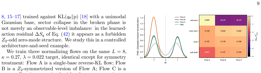
For two-dimensional lattice ϕ^4, a trained straight-flow teacher is not described by a local force basis alone. After the local transport basis, the residual separates into a zero-mode Binder component and a lowest-shell finite-k correlator component. The deflated zero-mode polynomial P_5(M;t) reduces the dominant Binder-tail component, while ϕ^⊥_{|n|^2=1} reduces the finite-k correlator component; wrong-parity, off-zero-mode, and random controls do not produce the same reductions. The same projection distinguishes other sampler classes: diffusion follows the force-resolvent ordering predicted by the free theory, reverse-KL normalizing-flow collapse appears as a forbidden odd zero-mode, and

What carries the argument

Operator bases fixed before the fit from symmetry, exact Gaussian path limits, finite-volume modes, and gauge covariance, applied to project trained field-space functions and isolate residual components that lower held-out errors.

If this is right

Diffusion samplers follow the force-resolvent ordering expected from free theory.
Reverse-KL normalizing flows produce a forbidden odd zero-mode residual.
Gauge-equivariant teachers align with Wilson-loop-force tangent directions.
The projection test is model-dependent in its basis choice but applies uniformly across sampler classes.

Where Pith is reading between the lines

These are editorial extensions of the paper, not claims the author makes directly.

The method could be extended to higher dimensions or other interactions by adapting the symmetry-derived bases to new finite-volume modes.
Sampler training algorithms might be modified to penalize specific residual sectors identified here, such as odd zero-mode components.
The separation into zero-mode and finite-k parts suggests that non-local effects in trained flows arise from distinct physical mechanisms rather than uniform underfitting.

Load-bearing premise

The selected operator bases are assumed to be complete enough that any residual reduction after projection reflects real physical components rather than gaps in the basis.

What would settle it

If the deflated zero-mode polynomial P_5(M;t) and ϕ^⊥_{|n|^2=1} fail to reduce held-out residuals more than wrong-parity or random controls, or if the residual does not separate into zero-mode and finite-k components after the local basis, the structured-component claim is falsified.

Figures

Figures reproduced from arXiv: 2605.11199 by Moxian Qian.

**Figure 2.** Figure 2: FIG. 2. Trained-teacher residual shell spectrum at [PITH_FULL_IMAGE:figures/full_fig_p007_2.png] view at source ↗

**Figure 3.** Figure 3: FIG. 3. Size transfer separates coefficients from operator classes. (a) Applying [PITH_FULL_IMAGE:figures/full_fig_p008_3.png] view at source ↗

**Figure 4.** Figure 4: FIG. 4. Diffusion force-resolvent ladder. The redundant [PITH_FULL_IMAGE:figures/full_fig_p008_4.png] view at source ↗

**Figure 5.** Figure 5: FIG. 5. Operator projection of the learned-action residual [PITH_FULL_IMAGE:figures/full_fig_p009_5.png] view at source ↗

**Figure 6.** Figure 6: FIG. 6. Gauge operator projection. Wilson-loop-force ladders (orange, connected) reduce the held-out matching residual; [PITH_FULL_IMAGE:figures/full_fig_p011_6.png] view at source ↗

**Figure 7.** Figure 7: FIG. 7. Rollout diagnostics on [PITH_FULL_IMAGE:figures/full_fig_p017_7.png] view at source ↗

**Figure 8.** Figure 8: FIG. 8. Six- [PITH_FULL_IMAGE:figures/full_fig_p018_8.png] view at source ↗

**Figure 9.** Figure 9: FIG. 9. Smoothness of projection-coefficient curves over the six- [PITH_FULL_IMAGE:figures/full_fig_p019_9.png] view at source ↗

**Figure 10.** Figure 10: FIG. 10. Cross-size comparison. The same operator classes appear at [PITH_FULL_IMAGE:figures/full_fig_p020_10.png] view at source ↗

**Figure 11.** Figure 11: reports the predefined L = 16 ladder used after the coefficient-transfer test. Six rungs are shown: the L4 baseline, zero-mode extensions through P5 and P7, soft-shell extensions through |n| 2 = 1 and |n| 2 = 2, and their combined basis. The result is channel-selective: P7 tightens the Binder channel, while ϕ ⊥ |n| 2=2 moves the next soft shell toward HMC. Residual HMC offsets remain after the final rung.… view at source ↗

**Figure 12.** Figure 12: FIG. 12. Wilson-loop observables as ratios to HMC. The trained gauge teachers are biased relative to HMC, and the [PITH_FULL_IMAGE:figures/full_fig_p022_12.png] view at source ↗

**Figure 13.** Figure 13: FIG. 13. Gauge coupling sweep. (a) U(1), [PITH_FULL_IMAGE:figures/full_fig_p024_13.png] view at source ↗

read the original abstract

Trained lattice samplers are usually judged by the ensembles they generate. Here we instead analyze the trained field-space function itself: a flow-matching velocity, a diffusion score, or a normalizing-flow action residual. We project these functions onto operator bases fixed before the fit, chosen from symmetry, exact Gaussian path limits, finite-volume modes, and gauge covariance. For two-dimensional lattice \(\phi^4\), a trained straight-flow teacher is not described by a local force basis alone. After the local transport basis, the residual separates into a zero-mode Binder component and a lowest-shell finite-\(k\) correlator component. The deflated zero-mode polynomial \(P_5(M;t)\) reduces the dominant Binder-tail component, while \(\phi^\perp_{|n|^2=1}\) reduces the finite-\(k\) correlator component; wrong-parity, off-zero-mode, and random controls do not produce the same reductions. The same projection distinguishes other sampler classes. Diffusion follows the force-resolvent ordering predicted by the free theory, reverse-KL normalizing-flow collapse appears as a forbidden odd zero-mode residual, and gauge-equivariant teachers are resolved by Wilson-loop-force tangent directions. The operator basis is model- and symmetry-dependent, but the test is common: project the trained field-space function and retain sectors that lower held-out residuals and pass the available controls.

Editorial analysis

A structured set of objections, weighed in public.

Desk editor's note, referee report, simulated authors' rebuttal, and a circularity audit. Tearing a paper down is the easy half of reading it; the pith above is the substance, this is the friction.

Desk Editor's Note private letter to a colleague

The paper gives a practical projection method to dissect trained sampler functions in lattice phi^4, but the operator basis completeness is still the key untested piece.

read the letter

The core new thing is projecting the trained velocity, score, or action residual onto symmetry-fixed operator bases to see what remains after subtracting a local force term. In 2D lattice phi^4 this cleanly splits the straight-flow residual into a zero-mode Binder component reduced by P_5(M;t) and a lowest-shell finite-k piece reduced by phi^perp at |n|^2=1, while wrong-parity and random controls do nothing. The same test then separates diffusion (which follows the expected resolvent ordering), reverse-KL flows (odd zero-mode leftover), and gauge-equivariant cases (Wilson-loop directions). That is a genuine addition; most prior checks only looked at generated ensembles or basic acceptance rates, not the internal function itself. The controls and the pre-fit choice of bases from Gaussian limits and finite-volume modes are the parts that feel honest and reproducible. The main soft spot is exactly the one the stress-test flags: without an explicit completeness argument or an exhaustive search inside the symmetry constraints, the observed residual drops could still come from missing higher operators rather than true physical decomposition. The abstract states the reductions but the full paper would need to show the actual held-out residual numbers, error bars, and how the projection is computed in practice before the separation can be taken as settled. Minor issues like basis dependence on the model are acknowledged in the text and do not undermine the test itself. This is for people already working on flow or diffusion models for lattice field theory who want a diagnostic beyond ensemble observables. It is narrow but concrete, and the method is simple enough that others could try it on their own trainers. I would send it to peer review; the idea is worth referee time even if the completeness question needs tightening in revision.

Referee Report

2 major / 2 minor

Summary. The paper introduces an 'operator spectroscopy' technique for dissecting trained lattice samplers (flow-matching velocity, diffusion score, or normalizing-flow action residual) by projecting them onto pre-fixed operator bases chosen from symmetry, exact Gaussian limits, finite-volume modes, and gauge covariance. For 2D lattice ϕ⁴ it claims that a straight-flow teacher cannot be captured by a local force basis alone; after that basis the residual decomposes into a dominant zero-mode Binder-tail component (reduced by the deflated polynomial P₅(M;t)) and a lowest-shell finite-k correlator component (reduced by ϕ^⊥_{|n|²=1}), while wrong-parity, off-zero-mode, and random controls do not produce comparable reductions. The same projection is shown to distinguish diffusion (force-resolvent ordering), reverse-KL flows (forbidden odd zero-mode residuals), and gauge-equivariant teachers (Wilson-loop-force directions).

Significance. If the central claims hold, the work supplies a concrete, symmetry-guided diagnostic that translates the internal structure of ML samplers back into the language of lattice field theory operators. This could improve interpretability, guide architecture choices, and help diagnose failures in high-dimensional sampling problems. The pre-fixed, non-circular basis construction is a methodological strength that distinguishes the approach from purely data-driven feature extraction.

major comments (2)

[Operator basis construction and projection procedure] The central claim that the residual 'separates into a zero-mode Binder component and a lowest-shell finite-k correlator component' (abstract and results) is load-bearing on the assumption that the chosen operators P₅(M;t) and ϕ^⊥_{|n|²=1} (plus their controls) form a sufficiently complete basis. The manuscript states that bases are fixed a priori from symmetry, Gaussian limits, finite-volume modes, and gauge covariance, but provides no explicit completeness argument, exhaustive enumeration within those constraints, or test against additional symmetry-allowed operators (e.g., higher-order zero-mode polynomials or other finite-volume shells). Without such a test, the observed residual reductions could arise from basis truncation rather than genuine physical decomposition.
[Results on residual decomposition and controls] The quantitative support for the reported residual reductions, control comparisons, and held-out performance (abstract claims of specific reductions and non-reductions) is not accompanied by error bars, sample sizes, or statistical significance tests in the presented results. This gap prevents confirmation that the differences between the target operators and the wrong-parity/off-zero-mode/random controls are robust rather than statistical fluctuations.

minor comments (2)

[Notation and definitions] Notation for the zero-mode polynomial P₅(M;t) should be clarified: the explicit time or flow-step dependence t is introduced without a definition of how it enters the deflation or the projection.
[Methods] The manuscript would benefit from a short table summarizing the operator bases used for each sampler class (straight flow, diffusion, reverse-KL, gauge-equivariant) together with the symmetry or limit that fixes each operator.

Simulated Author's Rebuttal

2 responses · 0 unresolved

We thank the referee for the positive evaluation of our work's significance and for the detailed comments. We provide point-by-point responses to the major comments and outline the revisions we will make to address them.

read point-by-point responses

Referee: [Operator basis construction and projection procedure] The central claim that the residual 'separates into a zero-mode Binder component and a lowest-shell finite-k correlator component' (abstract and results) is load-bearing on the assumption that the chosen operators P₅(M;t) and ϕ^⊥_{|n|²=1} (plus their controls) form a sufficiently complete basis. The manuscript states that bases are fixed a priori from symmetry, Gaussian limits, finite-volume modes, and gauge covariance, but provides no explicit completeness argument, exhaustive enumeration within those constraints, or test against additional symmetry-allowed operators (e.g., higher-order zero-mode polynomials or other finite-volume shells). Without such a test, the observed residual reductions could arise from basis truncation rather than genuine physical decomposition.

Authors: We agree that an explicit completeness argument would strengthen the presentation. The operator basis is constructed systematically from symmetry considerations, exact limits in the Gaussian theory, and finite-volume mode decomposition. The use of control operators (wrong parity, off-zero-mode, random) serves to demonstrate specificity: only the physically motivated operators produce significant residual reductions, while others do not. This suggests the decomposition is not an artifact of arbitrary truncation. Nevertheless, to address this concern, we will add a subsection discussing the rationale for the chosen basis, including why higher-order terms are expected to be subdominant based on the Gaussian limit, and include projections onto one additional higher-order zero-mode operator as a test. revision: partial
Referee: [Results on residual decomposition and controls] The quantitative support for the reported residual reductions, control comparisons, and held-out performance (abstract claims of specific reductions and non-reductions) is not accompanied by error bars, sample sizes, or statistical significance tests in the presented results. This gap prevents confirmation that the differences between the target operators and the wrong-parity/off-zero-mode/random controls are robust rather than statistical fluctuations.

Authors: We acknowledge this limitation in the current manuscript. Error bars and statistical tests were omitted for brevity. In the revised manuscript, we will include bootstrap-estimated error bars on all residual reduction plots, report the sample sizes explicitly, and perform statistical significance tests to assess the differences between target and control operators. This will confirm the robustness of the observed decompositions. revision: yes

Circularity Check

0 steps flagged

No significant circularity detected; analysis is empirical projection onto pre-fixed bases

full rationale

The paper fixes its operator bases prior to fitting, drawing them from symmetry, exact Gaussian path limits, finite-volume modes, and gauge covariance as stated in the abstract. It then performs projections of trained velocity/score/action functions onto these bases, measures residual reductions on held-out data, and applies controls (wrong-parity, off-zero-mode, random). This is an observational diagnostic procedure, not a closed derivation or prediction that reduces to its inputs by construction. No self-citations, self-definitional steps, fitted parameters renamed as predictions, or ansatz smuggling appear in the provided text. The central claim (residual separation into Binder and correlator components) is secured by explicit before-the-fit basis choice plus control tests rather than by tautology.

Axiom & Free-Parameter Ledger

0 free parameters · 0 axioms · 0 invented entities

Abstract provides no details on free parameters, axioms, or invented entities; the approach relies on pre-existing symmetry considerations and Gaussian limits from prior theory without introducing new fitted quantities or entities.

pith-pipeline@v0.9.0 · 5532 in / 1180 out tokens · 57155 ms · 2026-05-13T00:56:59.114423+00:00 · methodology

discussion (0)

Reference graph

Works this paper leans on

35 extracted references · 35 canonical work pages · 2 internal anchors

[1]

The free Gaussian reference is S0[ϕ] = 1 2 ϕT Kϕ, K >0,(A1) with covarianceK −1

Conventions The lattice field isϕ∈R V ,V=L 2. The free Gaussian reference is S0[ϕ] = 1 2 ϕT Kϕ, K >0,(A1) with covarianceK −1. An interacting target factorizes as S[ϕ] =S 0[ϕ] +S int[ϕ],(A2) with force F = −∇S = F0 + Fint, where F0 = −Kϕ and Fint = −∇Sint. In numerical projection K may be replaced by a positive regulated kernel Keff = m2 effI + 2κ(−∆) whe...

work page
[2]

Straight flow matching Independent endpointsϕ 0 ∼p 0,ϕ 1 ∼p 1, withϕ t = (1−t)ϕ 0 +tϕ 1, give the population FM minimizer v⋆ t (ϕ) =E[ϕ 1 −ϕ 0 |ϕ t =ϕ].(A3) Settingy=ϕ 1 and usingϕ 0 = (ϕ−ty)/(1−t), one finds v⋆ t (ϕ) = 1 1−t E[y|ϕ t =ϕ]−ϕ .(A4) Forp 0 =N(0, I), qt(y|ϕ) = 1 Zt(ϕ) exp −S[y]− 1 2(1−t) 2 ∥ϕ−ty∥ 2 .(A5) This formula is exact for any target. F...

work page
[3]

Variance-exploding diffusion For VE noisingx=y+σξ,ξ∼ N(0, I), qσ(y|x) = 1 Zσ(x) exp −S[y]− 1 2σ2 ∥x−y∥ 2 ,(A12) and Tweedie’s identity gives sσ(x) =∇ x logp σ(x) = 1 σ2 E[y|x]−x .(A13) ForS[y] = 1 2 yT Ky, the conditional is Gaussian with Cσ = (K+σ −2I) −1 =σ 2Rσ, m σ =R σx, Rσ = (I+σ 2K) −1.(A14) Thus s(0) σ (x) = 1 σ2 (Rσ −I)x=−R σKx=R σF0[x].(A15) For ...

work page
[4]

Near a Z2-symmetric critical region, the effective zero-mode potential takes the even Landau form Seff(M) =V(a 2M2 +a 4M4 +a 6M6 +· · ·)

Zero modes and soft shells The finite-volume zero mode is M = V −1P x ϕx. Near a Z2-symmetric critical region, the effective zero-mode potential takes the even Landau form Seff(M) =V(a 2M2 +a 4M4 +a 6M6 +· · ·). Since∂M/∂ϕ x = 1/V, the per-site force contains − ∂Seff ∂ϕx =−2a 2M−4a 4M3 −6a 6M5 − · · ·.(A18) This is the origin of the odd zero-mode tower. T...

work page
[5]

We compare raw coefficient SVD, operator-norm-normalized SVD, and sampler-level rank truncations

Coupling SVD protocol and rank summary For a basis withKoperators andN t time nodes, we stack C(n,j),a =c n(tj, κa). We compare raw coefficient SVD, operator-norm-normalized SVD, and sampler-level rank truncations. Rank-one rescaling is tested both as a reference-point rescaling and as an optimal SVD rank-one surface; in both cases it fails at the sampler...

work page
[6]

IV D are given in Table VIII

Held-out-κprediction table The full per-observable holdout- κ prediction numbers backing Sec. IV D are given in Table VIII. The HMC and UNet columns there use a separate 2000-sample HMC re-run and are not bit-identical to the canonical 8000-sample reference of Table II; the relative errors quoted in the main text are computed against this independent hold...

work page 2000
[7]

Smoothness of the coupling-coefficient surface The ϕ⊥ |n|2=1 coupling sweep is summarized in Fig. 8. The representative coefficient curves used to support the smoothness statement in Sec. IV D are shown in Fig. 9. 0.0 0.2 0.4 0.6 0.8 1.0 t 0.0 0.1 0.2 0.3 0.4 0.5 dϕ ⟂ |n|2 = 1(t, κ) NLO coefficient curve vs κ κ=0.22 κ=0.24 κ=0.26 κ=0.27 κ=0.28 κ=0.3 0.22 ...

work page
[8]

IV D is shown in Fig

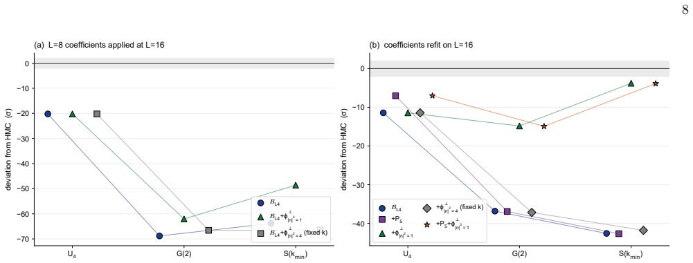
Cross-size visualization of operator-class transfer The cross-size visualization supporting the operator-class transfer statement of Sec. IV D is shown in Fig. 10. 20 L4 L4+P5 L4+ϕ ⟂ |n|2 =1 L4+P5+ϕ ⟂ |n|2 =1 L4 (L=16) L4+P5 L4+ϕ ⟂ |n|2 =1 L4+P5+ϕ ⟂ |n|2 =1 B6 (11 ops, full) −12 −10 −8 −6 −4 −2 0 2 ( ̄O − ̄OHMC)/σ U4 L=8 L=16 L4 L4+P5 L4+ϕ ⟂ |n|2 =1 L4+P5...

work page
[9]

Audit distribution

PredefinedL= 16NLO ladder Figure 11 reports the predefined L = 16 ladder used after the coefficient-transfer test. Six rungs are shown: the L4 baseline, zero-mode extensions through P5 and P7, soft-shell extensions through |n|2 = 1 and |n|2 = 2, and their combined basis. The result is channel-selective: P7 tightens the Binder channel, while ϕ⊥ |n|2=2 move...

work page
[10]

Mean plaquette and 1 ×2, 2 ×2 Wilson loops are shown in Fig

Wilson-loop observables and topology We sample from each trained teacher by a variance-exploding rollout (Heun integrator with Karras-style stochastic churn for U(1); pure Heun for SU(2)) and from each representation sampler by replacing the network output with the matched coefficient combination. Mean plaquette and 1 ×2, 2 ×2 Wilson loops are shown in Fi...

work page
[11]

VII E is reproduced as Table XIII

Architecture–projection overlap audit The architecture–projection overlap audit summarized in Sec. VII E is reproduced as Table XIII. 23 TABLE XIII. Architecture–projection overlap audit. Hard-coded primitives denote the symmetry-restricted output basis recorded for the checkpoint where available; the table should be read as an architecture audit, not as ...

work page
[12]

The Wilson-loop-force ladder is B0 = {VP }, B1 = {VP , VR}, B2 = {VP , VR, VP 2 }, B3 = {VP , VR, VP 2 , VPol}

U(1) coupling sweep For compact U(1) gauge theory with Wilson action [ 22] S[U] = −βP p cosθ p, we train the same gauge-equivariant DSM teacher at β∈ { 1.0, 2.0, 4.0, 6.0}, L = 8, using 4096 HMC samples and the same variance-exploding noise range as in the main text. The Wilson-loop-force ladder is B0 = {VP }, B1 = {VP , VR}, B2 = {VP , VR, VP 2 }, B3 = {...

work page
[13]

best control

SU(2) coupling sweep For SU(2) gauge theory with Wilson action S[U] = − β 2 P p Re TrUp, we train the same SU(2)-equivariant DSM teacher at β∈ { 1.5, 2.0, 3.0}, L = 6, with Wilson-loop-force ladder B0 = {VP }, B1 = {VP , VR}, B2 = {VP , VR, VadjP}. At every coupling the gauge-equivariance violation remains below ¯ϵgauge ≲ 4 × 10−4 across β∈ { 1.5, 2, 3}. ...

work page
[14]

Duane, A

S. Duane, A. D. Kennedy, B. J. Pendleton, and D. Roweth, Phys. Lett. B195, 216 (1987)

work page 1987
[15]

Metropolis, A

N. Metropolis, A. W. Rosenbluth, M. N. Rosenbluth, A. H. Teller, and E. Teller, J. Chem. Phys.21, 1087 (1953)

work page 1953
[16]

M. S. Albergo, G. Kanwar, and P. E. Shanahan, Phys. Rev. D100, 034515 (2019)

work page 2019
[17]

Kanwar, M

G. Kanwar, M. S. Albergo, D. Boyda, K. Cranmer, D. C. Hackett, S. Racani` ere, D. J. Rezende, and P. E. Shanahan, Phys. Rev. Lett.125, 121601 (2020)

work page 2020
[18]

K. A. Nicoli, C. J. Anders, L. Funcke, T. Hartung, K. Jansen, P. Kessel, S. Nakajima, and P. Stornati, Phys. Rev. Lett.126, 032001 (2021)

work page 2021
[19]

Lipman, R

Y. Lipman, R. T. Q. Chen, H. Ben-Hamu, M. Nickel, and M. Le, inInternational Conference on Learning Repre- sentations(2023)

work page 2023
[20]

X. Liu, C. Gong, and Q. Liu, inInternational Conference on Learning Representations(2023) arXiv:2209.03003

work page internal anchor Pith review Pith/arXiv arXiv 2023
[21]

Boyda, G

D. Boyda, G. Kanwar, S. Racani` ere, D. J. Rezende, M. S. Albergo, K. Cranmer, D. C. Hackett, and P. E. Shanahan, Phys. Rev. D103, 074504 (2021)

work page 2021
[22]

L. Wang, G. Aarts, and K. Zhou, J. High Energy Phys. 05, 060, arXiv:2309.17082

work page arXiv
[23]

Hyv¨ arinen, J

A. Hyv¨ arinen, J. Mach. Learn. Res.6, 695 (2005)

work page 2005
[24]

Y. Song, J. Sohl-Dickstein, D. P. Kingma, A. Kumar, S. Ermon, and B. Poole, inInternational Conference on Learning Representations(2021)

work page 2021
[25]

J. Ho, A. Jain, and P. Abbeel, inAdvances in Neural Information Processing Systems, Vol. 33 (2020) pp. 6840– 6851

work page 2020
[26]

Vincent, Neural Comput.23, 1661 (2011)

P. Vincent, Neural Comput.23, 1661 (2011)

work page 2011
[27]

Karras, M

T. Karras, M. Aittala, T. Aila, and S. Laine, inAdvances in Neural Information Processing Systems, Vol. 35 (2022) pp. 26565–26577

work page 2022
[28]

D. J. Rezende and S. Mohamed, inProceedings of the 32nd International Conference on Machine Learning, PMLR, 26 Vol. 37 (2015) pp. 1530–1538

work page 2015
[29]

L. Dinh, J. Sohl-Dickstein, and S. Bengio, inInterna- tional Conference on Learning Representations(2017) arXiv:1605.08803

work page internal anchor Pith review Pith/arXiv arXiv 2017
[30]

Papamakarios, E

G. Papamakarios, E. Nalisnick, D. J. Rezende, S. Mo- hamed, and B. Lakshminarayanan, J. Mach. Learn. Res. 22, 1 (2021)

work page 2021
[31]

Minka,Divergence measures and message passing, Tech

T. Minka,Divergence measures and message passing, Tech. Rep. MSR-TR-2005-173 (Microsoft Research, 2005)

work page 2005
[32]

T. S. Cohen and M. Welling, inProceedings of the 33rd International Conference on Machine Learning, PMLR, Vol. 48 (2016) pp. 2990–2999, arXiv:1602.07576

work page arXiv 2016
[33]

Binder, Z

K. Binder, Z. Phys. B43, 119 (1981)

work page 1981
[34]

Creutz, Phys

M. Creutz, Phys. Rev. D21, 2308 (1980)

work page 1980
[35]

K. G. Wilson, Phys. Rev. D10, 2445 (1974)

work page 1974