Recognition: 2 theorem links
· Lean TheoremAssessment of Time-of-Arrival Estimation Methods for Impact Detection in Isotropic Plates using Piezoceramic Sensors
Pith reviewed 2026-05-13 05:49 UTC · model grok-4.3
The pith
Time-of-arrival methods detect both symmetric and anti-symmetric Lamb wave modes from impacts on isotropic plates, with noise mainly disrupting the earliest arrivals.
A machine-rendered reading of the paper's core claim, the machinery that carries it, and where it could break.
Core claim
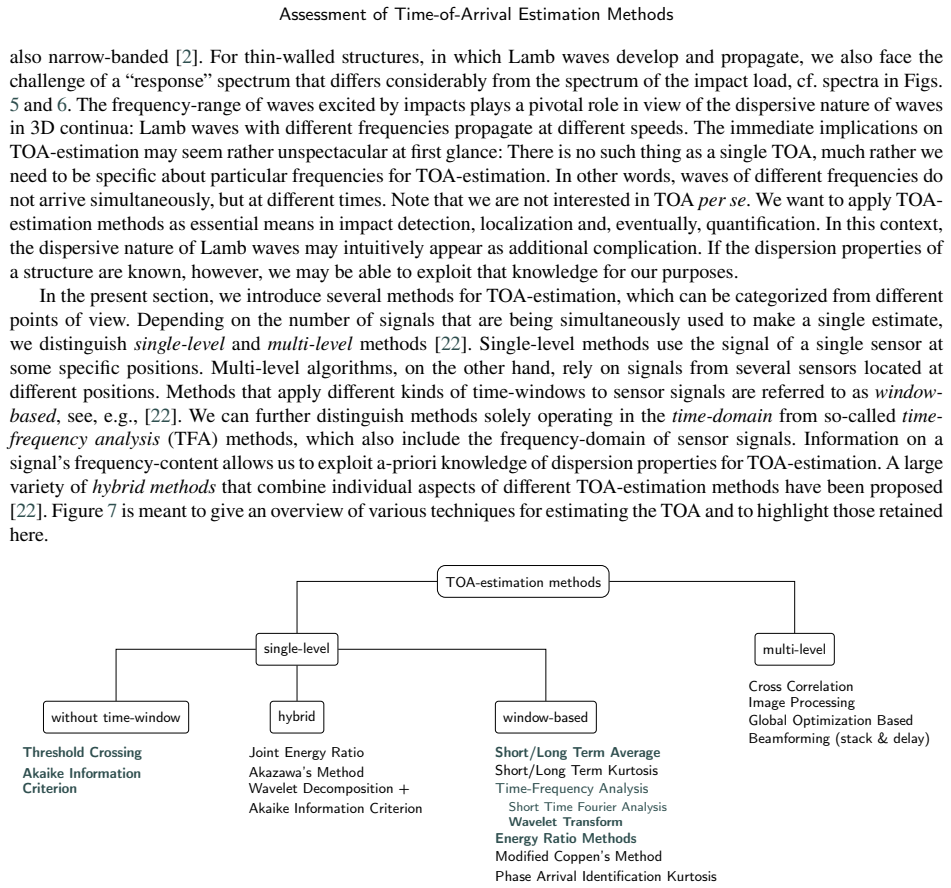
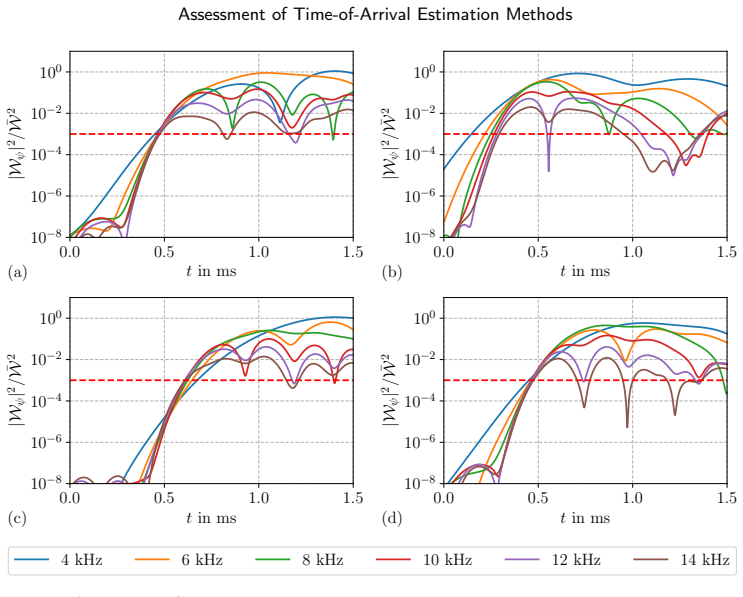
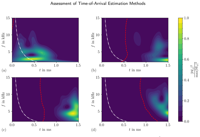
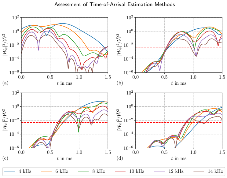
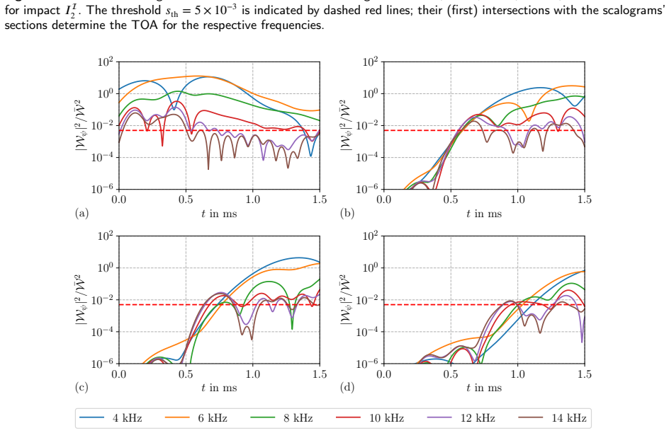
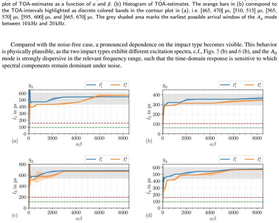
The paper establishes that threshold crossing, continuous wavelet transform, short/long term average, modified energy ratio, and Akaike information criterion methods can detect the fundamental Lamb wave modes from impact-induced waves monitored by piezoceramic sensors on isotropic plates. Under noise-free conditions nearly all methods capture both symmetric and anti-symmetric arrivals. Noise affects symmetric mode detection most, but anti-symmetric TOA can be estimated meaningfully with preprocessing or time-frequency methods. Novel elements are a frequency-domain threshold crossing inside the CWT framework for better robustness and accuracy, and using local minima of the AIC for the TOA of
What carries the argument
Time-of-arrival estimation algorithms applied to piezoceramic sensor signals recording impact-generated Lamb waves, including a frequency-domain threshold crossing extension to the continuous wavelet transform and local-minima consideration in the Akaike information criterion.
If this is right
- Nearly all assessed methods capture both symmetric and anti-symmetric fundamental Lamb wave mode arrivals under noise-free conditions.
- Noise primarily impairs detection of the earliest symmetric-mode arrivals.
- Meaningful anti-symmetric-mode TOA estimates remain obtainable through suitable preprocessing or time-frequency analysis even with noise.
- The new frequency-domain threshold crossing within the CWT framework improves both robustness and accuracy of TOA estimation.
- Considering local minima in the AIC proves effective for detecting the TOA of the fundamental symmetric mode.
Where Pith is reading between the lines
- These TOA techniques could support hybrid detection systems that switch between methods based on measured noise levels to maintain localization accuracy across varying impact conditions.
- Extending the assessment to anisotropic or layered plates would require incorporating direction-dependent group velocities into the signal models.
- The practical guidelines on method selection and preprocessing could guide sensor array design to minimize the impact of noise on early arrivals.
Load-bearing premise
The transient finite element simulations, after experimental calibration for excitation and dispersion, sufficiently represent real sensor signals for impacts at varying positions and force profiles, including under added noise.
What would settle it
Direct comparison of the methods' TOA outputs against known arrival times measured in controlled physical impact experiments on the same plate geometry, especially for signals with added noise levels matching the simulations.
Figures


read the original abstract
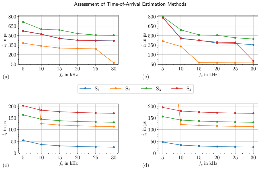
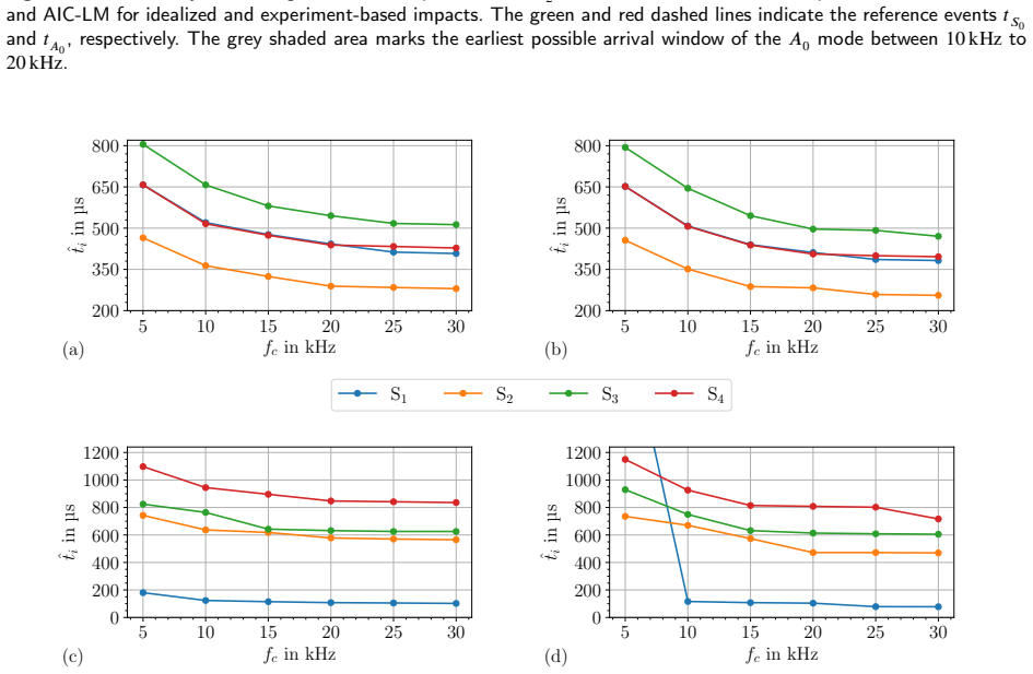
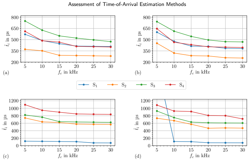
This work describes and assesses different methods for estimating the time-of-arrival (TOA) of impact-induced waves in isotropic plate-like structures. The methods considered include threshold crossing (TC), continuous wavelet transform (CWT), short/long term average (SLA), modified energy ratio (MER), and the Akaike information criterion (AIC). Their advantages, limitations, and sensitivities to method-specific parameters are systematically investigated. The assessment is based on synthetic data from transient finite element simulations that are experimentally calibrated with respect to excitation and dispersion characteristics. Wave propagation is monitored using piezoceramic patch sensors bonded to the plate surface, and robustness is evaluated for impacts of varying positions and force profiles, including noise-contaminated sensor signals in order to account for practically relevant measurement conditions. The results show that the methods are capable of detecting the fundamental Lamb wave modes, with nearly all capturing both the symmetric and anti-symmetric mode arrivals under noise-free conditions. In particular, noise primarily impairs the detection of the earliest symmetric-mode arrivals, while meaningful anti-symmetric-mode TOA-estimates can still be obtained by suitable preprocessing or time-frequency analysis. Besides, new contributions to the assessed TOA-estimation methods include a frequency-domain threshold crossing within the CWT framework that improves both robustness and accuracy of TOA-estimation, and the consideration of local minima in the AIC that proves effective for detecting the TOA of the fundamental symmetric mode. Beyond these findings, the research provides practical guidelines and insights into the specific characteristics of each assessed method, supporting accurate and reliable TOA-estimation for applications such as impact localization.
Editorial analysis
A structured set of objections, weighed in public.
Referee Report
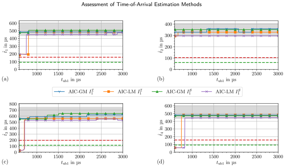
Summary. The manuscript assesses multiple time-of-arrival (TOA) estimation methods—threshold crossing (TC), continuous wavelet transform (CWT), short/long-term average (SLA), modified energy ratio (MER), and Akaike information criterion (AIC)—for detecting impact-induced Lamb waves in isotropic plates using piezoceramic sensors. Evaluation uses synthetic data from transient finite-element simulations experimentally calibrated for excitation amplitude and dispersion curves. Performance is examined across impact positions, force profiles, and additive noise. New contributions include a frequency-domain threshold-crossing variant inside the CWT framework and selection of local minima in the AIC for S0-mode detection. Results indicate that nearly all methods capture both S0 and A0 arrivals under noise-free conditions, noise primarily degrades earliest S0 detections while A0 estimates remain recoverable via preprocessing or time-frequency analysis, and the work supplies practical guidelines for method selection and tuning.
Significance. If the synthetic waveforms faithfully reproduce real piezoceramic sensor statistics under noise, the study supplies actionable guidelines for TOA estimation in structural-health-monitoring applications. The systematic empirical comparison on calibrated simulations, together with the two proposed algorithmic tweaks, could help practitioners improve robustness of impact localization. The low circularity (performance metrics are not derived from the same fitted parameters used to tune the methods) is a positive feature.
major comments (3)
- [Methods (synthetic data generation) and Results (noise-contaminated cases)] The central claims on noise robustness—that noise impairs S0 arrivals while meaningful A0 TOA estimates remain obtainable via preprocessing or CWT—are derived exclusively from synthetic noise added to FE traces calibrated only for excitation amplitude and dispersion curves. The manuscript does not demonstrate that the resulting time-frequency content, modal attenuation, sensor ringing, or non-stationary noise statistics match experimental piezoceramic outputs for the same impact locations and force histories (see abstract and the description of the synthetic-data pipeline). This is load-bearing for the reported detection rates and accuracy rankings.
- [Results and Discussion (proposed method variants)] The two new contributions—a frequency-domain threshold crossing inside the CWT and local-minima selection in the AIC—are asserted to improve robustness and accuracy, yet the manuscript provides neither quantitative error bars, statistical significance tests, nor cross-validation against held-out experimental traces to substantiate the magnitude of these gains over baseline implementations.
- [Methods] Parameter-sensitivity analysis, data-exclusion rules, and the precise definition of “meaningful” TOA estimates are not fully specified, preventing independent verification of the claimed systematic assessment and practical guidelines.
minor comments (2)
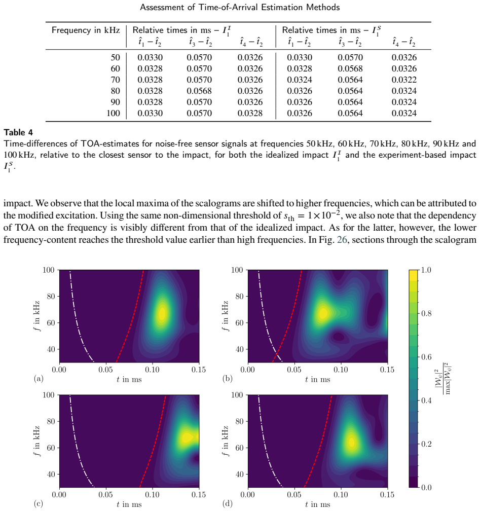
- [Figures] Figure captions should explicitly state the noise level (SNR) and impact parameters for each panel to improve readability.
- [Methods] Notation for the new CWT threshold-crossing variant should be introduced with a clear equation or pseudocode block.
Simulated Author's Rebuttal
We thank the referee for the constructive and detailed comments. We address each major point below and indicate the changes we will make to strengthen the manuscript.
read point-by-point responses
-
Referee: [Methods (synthetic data generation) and Results (noise-contaminated cases)] The central claims on noise robustness—that noise impairs S0 arrivals while meaningful A0 TOA estimates remain obtainable via preprocessing or CWT—are derived exclusively from synthetic noise added to FE traces calibrated only for excitation amplitude and dispersion curves. The manuscript does not demonstrate that the resulting time-frequency content, modal attenuation, sensor ringing, or non-stationary noise statistics match experimental piezoceramic outputs for the same impact locations and force histories (see abstract and the description of the synthetic-data pipeline). This is load-bearing for the reported detection rates and accuracy rankings.
Authors: We agree that the noise-robustness claims rest on additive Gaussian noise applied to FE traces calibrated solely for amplitude and dispersion. The study does not match experimental sensor ringing or non-stationary noise statistics. In revision we will (i) explicitly state these modeling assumptions in the Methods section, (ii) add a dedicated limitations paragraph in the Discussion, and (iii) rephrase the abstract and conclusions to present the results as indicative under the modeled conditions rather than experimentally validated. revision: yes
-
Referee: [Results and Discussion (proposed method variants)] The two new contributions—a frequency-domain threshold crossing inside the CWT and local-minima selection in the AIC—are asserted to improve robustness and accuracy, yet the manuscript provides neither quantitative error bars, statistical significance tests, nor cross-validation against held-out experimental traces to substantiate the magnitude of these gains over baseline implementations.
Authors: We will add error bars (standard deviation across noise realizations and impact positions) to all performance plots and tables. Where sample sizes permit, we will include simple statistical comparisons. Because the work uses only synthetic data, cross-validation on held-out experimental traces is not possible; we will note this limitation and identify experimental validation as future work. revision: partial
-
Referee: [Methods] Parameter-sensitivity analysis, data-exclusion rules, and the precise definition of “meaningful” TOA estimates are not fully specified, preventing independent verification of the claimed systematic assessment and practical guidelines.
Authors: We will expand the Methods section with a new subsection on parameter sensitivity, provide explicit data-exclusion criteria (e.g., TOA detections rejected when the estimated arrival falls outside the physically plausible window), and define “meaningful” TOA as an estimate whose absolute error is below a stated threshold relative to the known simulation arrival time. These additions will enable independent reproduction of the reported rankings and guidelines. revision: yes
Circularity Check
No circularity: empirical assessment on independent synthetic benchmarks
full rationale
The paper performs a comparative evaluation of TOA estimators (TC, CWT, SLA, MER, AIC) plus two proposed tweaks on transient FE-generated waveforms that were calibrated only for excitation amplitude and dispersion curves. All reported detection rates, accuracy rankings, and robustness statements are obtained by direct application of the methods to these fixed synthetic traces (with and without added noise). No performance metric is obtained by fitting a parameter to a subset of the assessment data and then re-using that parameter to compute the same or a closely related quantity. No self-citation chain is invoked to justify uniqueness or to close a derivation loop. The central claims therefore remain falsifiable against external experimental data and do not reduce to the input data by construction.
Axiom & Free-Parameter Ledger
axioms (1)
- domain assumption Transient finite-element simulations, once calibrated to experimental excitation and dispersion data, produce sensor signals representative of real piezoceramic measurements on isotropic plates.
Lean theorems connected to this paper
-
IndisputableMonolith/Foundation/RealityFromDistinction.leanreality_from_one_distinction unclearThe assessment is based on synthetic data from transient finite element simulations... methods include threshold crossing (TC), continuous wavelet transform (CWT), short/long term average (SLA), modified energy ratio (MER), and the Akaike information criterion (AIC).
-
IndisputableMonolith/Foundation/AlexanderDuality.leanalexander_duality_circle_linking unclearWe stay within the framework of linear elasticity... Navier-Cauchy equations... Rayleigh-Lamb equations
Reference graph
Works this paper leans on
-
[1]
Lamb, H., 1917. On waves in an elastic plate. Proceedings of the Royal Society of London. Series A, Containing Papers of a Mathematical and Physical Character 93, 114–128. doi:doi:10.1098/rspa.1917.0008
-
[2]
Structural health monitoring with piezoelectric wafer active sensors
Giurgiutiu, V., 2014. Structural health monitoring with piezoelectric wafer active sensors. 2. ed. ed., Academic Press/Elsevier, Amsterdam
work page 2014
-
[3]
Wave propagation in elastic solids
Achenbach, J.D., 1999. Wave propagation in elastic solids. volume 16 ofNorth Holland series in applied mathematics and mechanics. 7. impr ed., Elsevier, Amsterdam. doi:doi:10.1016/C2009-0-08707-8
-
[4]
Kundu, T., 2014. Acoustic source localization. Ultrasonics 54, 25–38. doi:doi:10.1016/j.ultras.2013.06.009
-
[5]
Journal of Sound and Vibration 329, 2384–2394
McLaskey,G.C.,Glaser,S.D.,Grosse,C.U.,2010.Beamformingarraytechniquesforacousticemissionmonitoringoflargeconcretestructures. Journal of Sound and Vibration 329, 2384–2394. doi:doi:10.1016/j.jsv.2009.08.037
-
[6]
Near-field beamforming analysis for acoustic emission source localization
He, T., Pan, Q., Liu, Y., Liu, X., Hu, D., 2012. Near-field beamforming analysis for acoustic emission source localization. Ultrasonics 52, 587–592. doi:doi:10.1016/j.ultras.2011.12.003
-
[7]
TheresponseofrectangularpiezoelectricsensorstoRayleighandLambultrasonicwaves
DiLanzaScalea,F.,Matt,H.,Bartoli,I.,2007. TheresponseofrectangularpiezoelectricsensorstoRayleighandLambultrasonicwaves. The Journal of the Acoustical Society of America 121, 175–187. doi:doi:10.1121/1.2400668
-
[8]
Ciampa, F., Meo, M., 2010. Acoustic emission source localization and velocity determination of the fundamental mode A0 using wavelet analysis and a Newton-based optimization technique. Smart Materials and Structures 19, 045027. doi:doi:10.1088/0964-1726/19/4/045027
-
[9]
Impactlocalizationincompositestructuresofarbitrarycrosssection
Ciampa,F.,Meo,M.,Barbieri,E.,2012. Impactlocalizationincompositestructuresofarbitrarycrosssection. StructuralHealthMonitoring: An International Journal 11, 643–655. doi:doi:10.1177/1475921712451951
-
[10]
Health monitoring of aerospace composite structures – active and passive approach
Staszewski, W.J., Mahzan, S., Traynor, R., 2009. Health monitoring of aerospace composite structures – active and passive approach. Composites Science and Technology 69, 1678–1685. doi:doi:10.1016/j.compscitech.2008.09.034
-
[11]
Impact source localization for composite structures under external dynamic loading condition
Jang, B.W., Lee, Y.G., Kim, C.G., Park, C.Y., 2015. Impact source localization for composite structures under external dynamic loading condition. Advanced Composite Materials 24, 359–374. doi:doi:10.1080/09243046.2014.917239
-
[12]
Merlo, E.M., Bulletti, A., Giannelli, P., Calzolai, M., Capineri, L., 2017. A novel differential time-of-arrival estimation technique for impact localization on carbon fiber laminate sheets. Sensors 17. doi:doi:10.3390/s17102270
-
[13]
Passive impact location estimation using piezoelectric sensors
Guyomar, D., Lallart, M., Monnier, T., Wang, X., Petit, L., 2009. Passive impact location estimation using piezoelectric sensors. Structural Health Monitoring: An International Journal 8, 357–367. doi:doi:10.1177/1475921709102090
-
[14]
Guyomar, D., Lallart, M., Petit, L., Wang, X.J., 2011. Impact localization and energy quantification based on the power flow: A low-power requirement approach. Journal of Sound and Vibration 330, 3270–3283. doi:doi:10.1016/j.jsv.2011.01.013
-
[15]
Impact detection in anisotropic materials using a time reversal approach
Ciampa, F., Meo, M., 2012. Impact detection in anisotropic materials using a time reversal approach. Structural Health Monitoring: An International Journal 11, 43–49. doi:doi:10.1177/1475921710395815
-
[16]
Impactlocalizationincomplexstructuresusinglaser-based time reversal
Park,B.,Sohn,H.,Olson,S.E.,DeSimio,M.P.,Brown,K.S.,Derriso,M.M.,2012. Impactlocalizationincomplexstructuresusinglaser-based time reversal. Structural Health Monitoring: An International Journal 11, 577–588. doi:doi:10.1177/1475921712449508
-
[17]
Atimereversalfocusingbasedimpactimagingmethodanditsevaluationoncomplexcomposite structures
Qiu,L.,Yuan,S.,Zhang,X.,Wang,Y.,2011. Atimereversalfocusingbasedimpactimagingmethodanditsevaluationoncomplexcomposite structures. Smart Materials and Structures 20, 105014. doi:doi:10.1088/0964-1726/20/10/105014
-
[18]
Tabian, I., Fu, H., Sharif Khodaei, Z., 2019. A convolutional neural network for impact detection and characterization of complex composite structures. Sensors 19. doi:doi:10.3390/s19224933
-
[19]
Anautomaticimpactmonitorforacompositepanelemployingsmartsensor technology
Haywood,J.,Coverley,P.T.,Staszewski,W.J.,Worden,K.,2005. Anautomaticimpactmonitorforacompositepanelemployingsmartsensor technology. Smart Materials and Structures 14, 265–271. doi:doi:10.1088/0964-1726/14/1/027
-
[20]
Impactdetectioninanaircraftcompositepanel—aneural-networkapproach
LeClerc,J.R.,Worden,K.,Staszewski,W.J.,Haywood,J.,2007. Impactdetectioninanaircraftcompositepanel—aneural-networkapproach. Journal of Sound and Vibration 299, 672–682. doi:doi:10.1016/j.jsv.2006.07.019
-
[21]
Seno, A.H., Sharif Khodaei, Z., Aliabadi, M.F.H., 2019. Passive sensing method for impact localisation in composite plates under simulated environmental and operational conditions. Mechanical Systems and Signal Processing 129, 20–36. doi:doi:10.1016/j.ymssp.2019.04.023
-
[22]
A review and appraisal of arrival-time picking methods for downhole microseismic data
Akram, J., Eaton, D.W., 2016. A review and appraisal of arrival-time picking methods for downhole microseismic data. Geophysics 81, KS71–KS91. doi:doi:10.1190/geo2014-0500.1
-
[23]
Time picking and random noise reduction on microseismic data
Han, L., Wong, J., Bancroft, J.C., 2009. Time picking and random noise reduction on microseismic data. CREWES Research Report , 1–13
work page 2009
-
[24]
Understanding and parameter setting of sta/lta trigger algorithm doi:doi:10.2312/GFZ.NMSOP-2_IS_8.1
Trnkoczy, A., . Understanding and parameter setting of sta/lta trigger algorithm doi:doi:10.2312/GFZ.NMSOP-2_IS_8.1
-
[25]
Detectionofthepointofimpactonastiffenedplatebytheacousticemissiontechnique
Kundu,T.,Das,S.,Jata,K.V.,2009. Detectionofthepointofimpactonastiffenedplatebytheacousticemissiontechnique. SmartMaterials and Structures 18, 035006. doi:doi:10.1088/0964-1726/18/3/035006. L. Grasboeck et al.:Preprint submitted to ElsevierPage 57 of 60 Assessment of Time-of-Arrival Estimation Methods
-
[26]
Anovelimpactidentificationalgorithmbasedonalinearapproximationwithmaximum entropy
Sanchez,N.,Meruane,V.,Ortiz-Bernardin,A.,2016. Anovelimpactidentificationalgorithmbasedonalinearapproximationwithmaximum entropy. Smart Materials and Structures 25, 095050. doi:doi:10.1088/0964-1726/25/9/095050
-
[27]
Determination of impact location on composite stiffened panels
Sharif Khodaei, Z., Ghajari, M., Aliabadi, M.H., 2012. Determination of impact location on composite stiffened panels. Smart Materials and Structures 21, 105026. doi:doi:10.1088/0964-1726/21/10/105026
-
[28]
Optimalsensorpositioningforimpactlocalizationinsmartcompositepanels
Mallardo,V.,Aliabadi,M.H.,SharifKhodaei,Z.,2013. Optimalsensorpositioningforimpactlocalizationinsmartcompositepanels. Journal of Intelligent Material Systems and Structures 24, 559–573. doi:doi:10.1177/1045389X12464280
-
[29]
Identification of the impact location on a plate using wavelets
Gaul, L., Hurlebaus, S., 1998. Identification of the impact location on a plate using wavelets. Mechanical Systems and Signal Processing 12, 783–795. doi:doi:10.1006/mssp.1998.0163
-
[30]
Hamstad, M., O’Gallagher, A., 2005. Effects of noise on lamb-mode acoustic-emission arrival times determined by wavelet transform URL: https://tsapps.nist.gov/publication/get_pdf.cfm?pub_id=50139
work page 2005
-
[31]
A wavelet tour of signal processing: The Sparse way
Mallat, S.G., 2009. A wavelet tour of signal processing: The Sparse way. 3.ed. ed., Elsevier /Academic Press, Amsterdam. doi:doi:10.1016/B978-0-12-374370-1.00002-1
-
[32]
Dris, E.Y., Drai, R., Bentahar, M., Berkani, D., 2020. Adaptive algorithm for estimating and tracking the location of multiple impacts on a plate-like structure. Research in Nondestructive Evaluation 31, 1–23. doi:doi:10.1080/09349847.2019.1617913
-
[33]
Impact identification on a sandwich plate from wave propagation responses
Meo, M., Zumpano, G., Piggott, M., Marengo, G., 2005. Impact identification on a sandwich plate from wave propagation responses. Composite Structures 71, 302–306. doi:doi:10.1016/j.compstruct.2005.09.028
-
[34]
Automatictimepickingoffirstarrivalsonnoisymicroseismicdata
Wong,J.,Han,L.,Bancroft,J.C.,Stewart,R.R.,2009. Automatictimepickingoffirstarrivalsonnoisymicroseismicdata. CSEGConference Abstracts
work page 2009
-
[35]
VanDecar,J.C.,Crosson,R.S.,1990. Determinationofteleseismicrelativephasearrivaltimesusingmulti-channelcross-correlationandleast squares. Bulletin of the Seismological Society of America 80, 150–169
work page 1990
-
[36]
De Meersman, K., Kendall, J.M., van der Baan, M., 2009. The 1998 valhall microseismic data set: An integrated study of relocated sources, seismic multiplets, and s-wave splitting. GEOPHYSICS 74, B183–B195. doi:doi:10.1190/1.3205028
-
[37]
First-break timing: Arrival onset times by direct correlation
Molyneux, J.B., Schmitt, D.R., 1999. First-break timing: Arrival onset times by direct correlation. GEOPHYSICS 64, 1492–1501. doi:doi:10.1190/1.1444653
-
[38]
Automatic p phase picking using maximum kurtosis and𝜅-statistics criteria
Saragiotis, C.D., Hadjileontiadis, L.J., Rekanos, I.T., Panas, S.M., 2004. Automatic p phase picking using maximum kurtosis and𝜅-statistics criteria. IEEE Geoscience and Remote Sensing Letters 1, 147–151. doi:doi:10.1109/LGRS.2004.828915
-
[39]
Lokajíćek, T., Klíma, K., 2006. A first arrival identification system of acoustic emission (AE) signals by means of a high-order statistics approach. Measurement Science and Technology 17, 2461–2466. doi:doi:10.1088/0957-0233/17/9/013
-
[40]
Determiningultrasoundarrivaltimebyhhtandkurtosisinwindspeedmeasurement
Liu,S.,Li,Z.,Wu,T.,Zhang,W.,2021. Determiningultrasoundarrivaltimebyhhtandkurtosisinwindspeedmeasurement. Electronics10,
work page 2021
-
[41]
doi:doi:10.3390/electronics10010093
-
[42]
Automatic phase pickers: Their present use and future prospects
Allen, R., 1982. Automatic phase pickers: Their present use and future prospects. Bulletin of the Seismological Society of America 72, S225–S242. doi:doi:10.1785/BSSA07206B0225
-
[43]
Acousticemissionlocalizationinthinmulti-layerplatesusingfirst-arrivaldetermination
Sedlak,P.,Hirose,Y.,Enoki,M.,2013. Acousticemissionlocalizationinthinmulti-layerplatesusingfirst-arrivaldetermination. Mechanical Systems and Signal Processing 36, 636–649. doi:doi:10.1016/j.ymssp.2012.11.008
-
[44]
Impact source localisation in aerospace composite structures
de Simone, M.E., Ciampa, F., Boccardi, S., Meo, M., 2017. Impact source localisation in aerospace composite structures. Smart Materials and Structures 26, 125026. doi:doi:10.1088/1361-665X/aa973e
-
[45]
Hou, D., Huang, K., Qi, X., Wang, W., Bi, X., Kong, J., Chang, Y., Zhao, L., Hu, N., 2025. Arrival time detection of ae signals using multi-threshold wavelet denoising and improved aic for composites damage localization. Mechanical Systems and Signal Processing 237, 113080. doi:doi:10.1016/j.ymssp.2025.113080
-
[46]
Barile, C., Casavola, C., Pappalettera, G., Paramsamy Kannan, V., 2025. Investigation of an improved time of arrival detection method for acoustic emission signals and its applications to damage characterisation in composite materials. Mechanical Systems and Signal Processing 223, 111906. doi:doi:10.1016/j.ymssp.2024.111906
-
[47]
First-break refraction event picking and seismic data trace editing using neural networks
McCormack, M.D., Zaucha, D.E., Dushek, D.W., 1993. First-break refraction event picking and seismic data trace editing using neural networks. GEOPHYSICS 58, 67–78. doi:doi:10.1190/1.1443352
-
[48]
Automatic picking of seismic arrivals in local earthquake data using an artificial neural network
Dai, H., MacBeth, C., 1995. Automatic picking of seismic arrivals in local earthquake data using an artificial neural network. Geophysical Journal International 120, 758–774. doi:doi:10.1111/j.1365-246X.1995.tb01851.x
-
[49]
Deep learning approaches for robust time of arrival estimation in acoustic emission monitoring
Zonzini, F., Bogomolov, D., Dhamija, T., Testoni, N., de Marchi, L., Marzani, A., 2022. Deep learning approaches for robust time of arrival estimation in acoustic emission monitoring. Sensors (Basel, Switzerland) 22. doi:doi:10.3390/s22031091
-
[50]
Stoica, P., Selen, Y., 2004. Model-order selection. IEEE Signal Processing Magazine 21, 36–47. doi:doi:10.1109/MSP.2004.1311138
-
[51]
Aprocedureforthemodelingofnon-stationarytimeseries
Kitagawa,G.,Akaike,H.,1978. Aprocedureforthemodelingofnon-stationarytimeseries. AnnalsoftheInstituteofStatisticalMathematics 30, 351–363. doi:doi:10.1007/BF02480225
-
[52]
Altenbach, H., 2015. Kontinuumsmechanik. Springer Berlin Heidelberg, Berlin, Heidelberg. doi:doi:10.1007/978-3-662-47070-1
-
[53]
Tipler, P.A., Llewellyn, R., 2012. Modern physics. 6. ed. ed., Freeman, New York
work page 2012
- [54]
-
[55]
Lighthill, M.J., 1965. Group velocity. IMA Journal of Applied Mathematics 1, 1–28. doi:doi:10.1093/imamat/1.1.1
- [56]
-
[57]
Ansys Help, .https://ansyshelp.ansys.com/
-
[58]
A method of computation for structural dynamics
Newmark, N.M., 1959. A method of computation for structural dynamics. Journal of the Engineering Mechanics Division Vol. 85, 67–94
work page 1959
-
[59]
Handbookofnondestructiveevaluation:RodrickRules.volume2ofMcGraw-HillHandbooks
Hellier,C.J.,2001. Handbookofnondestructiveevaluation:RodrickRules.volume2ofMcGraw-HillHandbooks. McGraw-Hill,NewYork
work page 2001
- [60]
- [61]
-
[62]
Construction and Building Materials 273, 121706
Cheng,L.,Xin,H.,Groves,R.M.,Veljkovic,M.,2021.Acousticemissionsourcelocationusinglambwavepropagationsimulationandartificial neural network for I-shaped steel girder. Construction and Building Materials 273, 121706. doi:doi:10.1016/j.conbuildmat.2020.121706
-
[63]
Impactdamagelocationincompositestructuresusingoptimizedsensortriangulationprocedure
Coverley,P.T.,Staszewski,W.J.,2003. Impactdamagelocationincompositestructuresusingoptimizedsensortriangulationprocedure. Smart Materials and Structures 12, 795–803. doi:doi:10.1088/0964-1726/12/5/017
-
[64]
Shearer, P.M., 2011. Introduction to seismology. 2. ed., repr. with corr ed., Cambridge Univ. Press, Cambridge
work page 2011
-
[65]
Cohen, L., 1995. Time-frequency analysis. Prentice Hall signal processing series, Prentice Hall PTR, Upper Saddle River, NJ
work page 1995
-
[66]
Billingsley, P., 1995. Probability and measure. A Wiley-Interscience publication. 3. ed. ed., Wiley, New York, NY
work page 1995
-
[67]
Estimating computational noise
Moré, J.J., Wild, S.M., 2011. Estimating computational noise. SIAM Journal on Scientific Computing 33, 1292–1314. doi:doi:10.1137/100786125
-
[68]
Bennett,W.R.,1948. Spectraofquantizedsignals. BellSystemTechnicalJournal27,446–472. doi:doi:10.1002/j.1538-7305.1948.tb01340.x
-
[69]
doi:doi:10.1016/j.ymssp.2026.114105
Jana,S.,Kapuria,S.,2026.Fastandaccuratedecompositionofoverlappinglambwavemodesinmetallicandcompositestructures.Mechanical Systems and Signal Processing 250, 114105. doi:doi:10.1016/j.ymssp.2026.114105
-
[70]
Gabor, D., 1946. Theory of communication. part 1: The analysis of information. Journal of the Institution of Electrical Engineers - Part III: Radio and Communication Engineering 93, 429–441. doi:doi:10.1049/ji-3-2.1946.0074
-
[71]
Arts, L.P.A., van den Broek, E.L., 2022. The fast continuous wavelet transformation (fCWT) for real-time, high-quality, noise-resistant time–frequency analysis. Nature Computational Science 2, 47–58. doi:doi:10.1038/s43588-021-00183-z
-
[72]
Wavelets and signal processing
Rioul, O., Vetterli, M., 1991. Wavelets and signal processing. IEEE Signal Processing Magazine 8, 14–38. doi:doi:10.1109/79.91217
-
[73]
Optimal Mother Wavelet Selection for Lamb Wave Analyses
Li, F., Meng, G., Kageyama, K., Su, Z., Ye, L., 2009. Optimal Mother Wavelet Selection for Lamb Wave Analyses. Journal of Intelligent Material Systems and Structures 20, 1147–1161. doi:doi:10.1177/1045389X09102562
-
[74]
Damageidentificationbasedonridgesandmaximalinesofthewavelettransform
Haase,M.,Widjajakusuma,J.,2003. Damageidentificationbasedonridgesandmaximalinesofthewavelettransform. InternationalJournal of Engineering Science 41, 1423–1443. doi:doi:10.1016/S0020-7225(03)00026-0
-
[75]
SciPy 1.0: fundamental algorithms for scientific computing in Python
Virtanen, P., Gommers, R., Oliphant, T.E., Haberland, M., Reddy, T., Cournapeau, D., Burovski, E., Peterson, P., Weckesser, W., Bright, J., van der Walt, S.J., Brett, M., Wilson, J., Millman, K.J., Mayorov, N., Nelson, A.R.J., Jones, E., Kern, R., Larson, E., Carey, C.J., Polat, I., Feng, Y., Moore, E.W., VanderPlas, J., Laxalde, D., Perktold, J., Cimrman...
-
[76]
Torrence, C., Compo, G.P., 1998. A practical guide to wavelet analysis. Bulletin of the American Meteorological Society 79, 61–78. doi:doi:10.1175/1520-0477(1998)079<0061:APGTWA>2.0.CO;2
-
[77]
A new look at the statistical model identification
Akaike, H., 1974. A new look at the statistical model identification. IEEE Transactions on Automatic Control 19, 716–723. doi:doi:10.1109/TAC.1974.1100705
-
[78]
Sleeman, R., van Eck, T., 1999. Robust automatic p-phase picking: an on-line implementation in the analysis of broadband seismogram recordings. Physics of the Earth and Planetary Interiors 113, 265–275. doi:doi:10.1016/S0031-9201(99)00007-2
-
[79]
Probability, random processes, and statistical analysis
Kobayashi, H., Mark, B.L., Turin, W., 2012. Probability, random processes, and statistical analysis. Cambridge University Press, Cambridge and New York
work page 2012
-
[80]
Comparisonofmanualandautomaticonsettimepicking
Leonard,M.,2000. Comparisonofmanualandautomaticonsettimepicking. BulletinoftheSeismologicalSocietyofAmerica90,1384–1390. doi:doi:10.1785/0120000026
discussion (0)
Sign in with ORCID, Apple, or X to comment. Anyone can read and Pith papers without signing in.