arxiv: 2605.11911 · v1 · submitted 2026-05-12 · 💻 cs.LG

Recognition: 1 theorem link

· Lean Theorem

Understanding Sample Efficiency in Predictive Coding

Gaspard Oliviers , Elene Lominadze , Rafal Bogacz

Authors on Pith no claims yet

Pith reviewed 2026-05-13 07:43 UTC · model grok-4.3

classification 💻 cs.LG

keywords predictive codingbackpropagationsample efficiencytarget alignmentdeep linear networksmachine learning

0 comments

The pith

Predictive coding produces weight updates that align more closely with output errors than backpropagation, yielding higher sample efficiency.

A machine-rendered reading of the paper's core claim, the machinery that carries it, and where it could break.

The paper measures learning efficiency by how closely a weight update changes the network output in the direction of the output prediction error. It derives exact expressions for this alignment in deep linear networks and shows that predictive coding consistently produces higher alignment than backpropagation. The difference is largest in deep narrow networks and in networks that have already been pre-trained. Experiments confirm that the predicted efficiency advantage appears in practice even when networks contain nonlinear activations.

Core claim

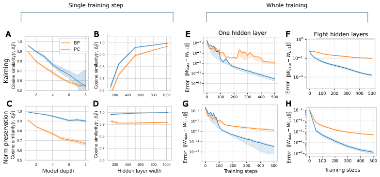
In deep linear networks the change in output produced by a predictive-coding update lies closer to the output prediction error than the change produced by a backpropagation update. Closed-form expressions for the alignment angle are obtained by tracking the forward and backward signals through the layers; these expressions show that predictive coding reaches the maximum possible alignment when its learning rates satisfy a simple ratio condition derived from the network's singular values.

What carries the argument

Target alignment, the cosine of the angle between the output change induced by a weight update and the output prediction error.

If this is right

Fewer training samples are needed to reach a given performance level when using predictive coding instead of backpropagation.
The efficiency gap widens as depth increases and narrows as width increases.
Pre-training further increases the relative advantage of predictive coding.
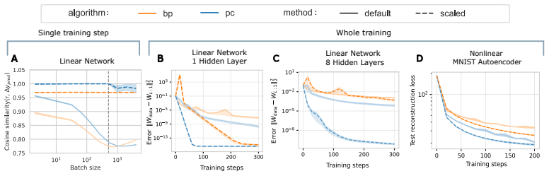
Optimal alignment in predictive coding occurs only when layer-wise learning rates obey a specific ratio determined by the singular values of the weight matrices.

Where Pith is reading between the lines

These are editorial extensions of the paper, not claims the author makes directly.

The same alignment analysis could be applied to other local learning rules that avoid a global backward pass.
In settings where data are scarce, such as continual learning or few-shot adaptation, predictive coding may reduce the number of required examples.
Hardware implementations that support only local updates could exploit the higher alignment to reach target performance with lower energy cost.

Load-bearing premise

The exact formulas assume a deep linear network; the advantage in nonlinear networks rests on empirical observation rather than proof.

What would settle it

Train a deep linear network of depth 10 and width 5 with both methods on a regression task and measure whether predictive coding's target alignment remains higher than backpropagation's throughout training.

Figures

Figures reproduced from arXiv: 2605.11911 by Elene Lominadze, Gaspard Oliviers, Rafal Bogacz.

**Figure 1.** Figure 1: Target alignment. (A) Deep Linear Network (DLN) used in the toy model has one input neuron, one hidden neuron and two output neurons y1 and y2. All weights are initialised to be one. (B) Evolution of a DLN’s predictions yˆi during training with BP and PC. The network receives an input of x = 1 with a target output of y = [−1, 1]. Training is carried out separately using PC and BP until the model output mat… view at source ↗

**Figure 2.** Figure 2: Target Alignment in Predictive Coding (PC) and Backpropagation (BP). (A-D) Target alignment of BP (orange) and PC (blue) after one training step for a deep linear network with different architectures and initialisations. The dashed grey lines in panels B and D denote square networks. (E, G) Training dynamics of linear BP and PC under different initialisations and a batch size of 64. The models are square w… view at source ↗

**Figure 3.** Figure 3: Rescaling learning rate for online learning. (A) Target Alignment as a function of the condition number of the weight matrix for four models, BP, PC and their rescaled counterparts. (B) Training dynamics of a square linear network with 20 units per layer. (C) Training of the same square network with 8 hidden layers. Curves are averaged over 10 runs. (D) Nonlinear autoencoder with 3 hidden layers and traine… view at source ↗

**Figure 4.** Figure 4: Weight update rescaling for batch training (A) Target Alignment as a function of the batch size for four models, BP (solid orange), PC (solid blue) and their rescaled counterparts (dashed). (B) Training dynamics of the models trained with a batch size of 64 for a 1 hidden layer square linear network with 20 units per layer, as well as its deeper counterpart with 8 hidden layers (C). (D) Nonlinear autoencod… view at source ↗

**Figure 5.** Figure 5: Target alignment comparison: ResNets vs. DLNs. Target alignment as a function of network depth for BP and PC in linear residual networks and deep linear networks. ResNets achieve slightly higher target alignment than equivalent DLNs due to improved weight conditioning from skip connections. PC outperforms BP in both architectures, with the advantage growing with network depth as BP interference accumulates… view at source ↗

**Figure 6.** Figure 6: demonstrates that layer-specific learning rate scaling enables perfect alignment in ResNets. With αl = 1/(x ∗⊤ l−1x ∗ l−1 ), PC achieves target alignment of 1.0 independently of network depth, confirming that the theoretical guarantee extends to skip-connected architectures. 2 3 4 5 6 Network Depth 0.65 0.70 0.75 0.80 0.85 0.90 0.95 1.00 Target Alignment Layer scaling removes interference Perfect Alignment… view at source ↗

**Figure 7.** Figure 7: shows training curves and learning rate sweeps for varying widths (15, 20, 40) and initialisations (Kaiming Uniform and Norm-Preservation) in a network with 20 input and output units and one hidden layer. Both PC and BP are trained for 500 steps with a batch size of 64, and the results are averaged over 10 seeds. The two middle figures on the left (within the “Training Curves for Varying Widths”) panel ar… view at source ↗

**Figure 8.** Figure 8: Training curves and learning rate sweeps for scaled and default versions of PC and BP during online as well as batch learning. For online learning, learning rate rescaling provides effectively no benefits compared to the default algorithms. For batch training, however, rescaled PC consistently outperforms all other models. Comparison between default PC and BP again shows that PC consistently performs bette… view at source ↗

**Figure 9.** Figure 9: Training trajectories and learning rate sweeps for a Nonlinear Autoencoder. Comparison of training trajectories for BP, PC and their rescaled versions for online learning and batch learning. PC outperforms BP in both cases, though the rescaled algorithms only benefit from larger batch sizes. For larger batch sizes, rescaled PC weight updates approach natural gradients. 25 [PITH_FULL_IMAGE:figures/full_fi… view at source ↗

**Figure 10.** Figure 10: Training trajectories and learning rate sweeps for networks with 8 hidden layers. Comparison between default/scaled BP and PC for deep networks with 8 hidden layers. For these networks, the same trend emerges as for 1 hidden layer counterparts - benefits offered by rescaling can be observed mostly when we increase the batch size to 64. Learning rate sweeps are performed over the interval 10−5 − 100 , samp… view at source ↗

read the original abstract

Predictive Coding (PC) is an influential account of cortical learning. Much of recent work has focused on comparing PC to Backpropagation (BP) to find whether PC offers any advantages. Small scale experiments show that PC enables learning that is more sample efficient and effective in many contexts, though a thorough theoretical understanding of the phenomena remains elusive. To address this, we quantify the efficiency of learning in BP and PC through a metric called ``target alignment'', which measures how closely the change in the output of the network is aligned to the output prediction error. We then derive and empirically validate analytical expressions for target alignment in Deep Linear Networks. We show that learning in PC is more efficient than BP, which is especially pronounced in deep, narrow and pre-trained networks. We also derive exact conditions for guaranteed optimal target alignment in PC and validate our findings through experiments. We study full training trajectories of linear and non-linear models, and find the predicted benefits of PC persist in practice even when some assumptions are violated. Overall, this work provides a mechanistic understanding of the higher learning efficiency observed for PC over BP in previous works, and can guide how PC should be parametrised to learn most effectively.

Editorial analysis

A structured set of objections, weighed in public.

Desk editor's note, referee report, simulated authors' rebuttal, and a circularity audit. Tearing a paper down is the easy half of reading it; the pith above is the substance, this is the friction.

Desk Editor's Note private letter to a colleague

The paper derives closed-form target alignment for PC vs BP in deep linear networks and shows a PC edge, but the nonlinear efficiency claim stays empirical.

read the letter

The main point is that they introduce target alignment as a measure of how well updates move the output toward the error, then derive exact expressions for it in deep linear networks. This lets them show PC produces better alignment than backprop, with the gap largest in deep, narrow, or pretrained cases, plus conditions that guarantee optimal alignment under PC. They also run full trajectories and check that the advantage shows up in nonlinear models too. That analytical step on linear dynamics is the actual new piece and it is done cleanly from the network equations without obvious circularity. The empirical extension to nonlinear nets is a fair check that the benefit survives when the assumptions break. The soft spot is the scope: all the closed forms and optimality conditions are linear-specific, so the mechanistic account for why PC should be more sample-efficient does not yet cover the nonlinear regime where most practical interest lies. The nonlinear results are reported as persisting, but without a parallel derivation they remain observations rather than explained. Experimental details are not visible here, so controls for initialization, depth, and width choices cannot be judged directly. This is useful for anyone working on alternative learning rules or cortical models who wants a quantitative handle on sample efficiency differences. The linear analysis gives something concrete to build on even if the general claim needs more work. I would send it to peer review; the derivations are substantive enough to merit referee input on the math and on how far the story can be pushed beyond linearity.

Referee Report

0 major / 3 minor

Summary. The paper introduces target alignment as a metric for sample efficiency and derives closed-form analytical expressions for it in deep linear networks under both backpropagation (BP) and predictive coding (PC). It shows that PC yields higher target alignment than BP, with the advantage most pronounced in deep, narrow, and pre-trained networks, and provides exact conditions guaranteeing optimal alignment in PC. These derivations are empirically validated on linear models; full training trajectories are then studied for both linear and nonlinear networks, where the efficiency benefits of PC are reported to persist even when linearity assumptions are violated.

Significance. If the results hold, the work supplies a mechanistic account of PC's sample-efficiency advantage over BP that is grounded in explicit derivations rather than post-hoc fitting. The closed-form expressions and exact optimality conditions for the linear case constitute a clear strength, as they yield falsifiable predictions about network depth, width, and initialization. The empirical demonstration that benefits survive in nonlinear regimes broadens the practical relevance for biologically inspired learning algorithms.

minor comments (3)

[§3.2] §3.2: The transition from the linear-network derivation to the nonlinear experiments would benefit from an explicit statement of which quantities (e.g., the alignment metric itself) remain unchanged versus which are only observed empirically.
[Figure 3] Figure 3 caption: the legend does not indicate whether the pre-trained curves start from the same initialization distribution as the from-scratch curves; this affects interpretation of the depth and width effects.
[Table 2] Table 2: the reported R² values for the PC alignment fit lack confidence intervals or degrees of freedom, making it difficult to judge how tightly the closed-form expression matches the simulated trajectories.

Simulated Author's Rebuttal

0 responses · 0 unresolved

We are grateful to the referee for the positive and accurate summary of our work, as well as the recommendation for minor revision. We note that no specific major comments were provided in the report. Accordingly, our point-by-point responses are not applicable, and we have no standing objections. We will proceed with minor revisions to the manuscript as appropriate.

Circularity Check

0 steps flagged

Derivations of target alignment in deep linear networks are first-principles calculations with no reduction to inputs by construction.

full rationale

The paper defines target alignment as a metric measuring alignment between output change and prediction error, then derives closed-form analytical expressions for this quantity specifically in deep linear networks. These steps are presented as direct calculations on network dynamics and learning rules rather than any fitted parameter being renamed as a prediction, self-definitional loop, or load-bearing self-citation. No equations reduce the claimed PC > BP efficiency advantage to the same quantities used to define alignment. The persistence of benefits in nonlinear cases is noted only empirically without a claimed derivation, but this does not create circularity in the linear analysis itself. The work therefore remains self-contained against external benchmarks with independent analytical content.

Axiom & Free-Parameter Ledger

0 free parameters · 1 axioms · 0 invented entities

Central claim rests on the definition of target alignment and the assumption that linear-network dynamics yield tractable closed-form expressions; no free parameters or invented entities are mentioned in the abstract.

axioms (1)

domain assumption Deep linear networks admit closed-form expressions for weight-update effects on output alignment
Invoked to derive target alignment for both PC and BP.

pith-pipeline@v0.9.0 · 5504 in / 1171 out tokens · 47271 ms · 2026-05-13T07:43:05.423763+00:00 · methodology

discussion (0)

Lean theorems connected to this paper

Citations machine-checked in the Pith Canon. Every link opens the source theorem in the public Lean library.

IndisputableMonolith/Cost/FunctionalEquation.lean washburn_uniqueness_aczel unclear

?

unclear
Relation between the paper passage and the cited Recognition theorem.

We derive closed-form expressions for the change in prediction induced by PC and BP updates in DLNs and compare their target alignment.

What do these tags mean?

matches: The paper's claim is directly supported by a theorem in the formal canon.
supports: The theorem supports part of the paper's argument, but the paper may add assumptions or extra steps.
extends: The paper goes beyond the formal theorem; the theorem is a base layer rather than the whole result.
uses: The paper appears to rely on the theorem as machinery.
contradicts: The paper's claim conflicts with a theorem or certificate in the canon.
unclear: Pith found a possible connection, but the passage is too broad, indirect, or ambiguous to say the theorem truly supports the claim.

Reference graph

Works this paper leans on

27 extracted references · 27 canonical work pages

[1]

R. P. N. Rao and D. H. Ballard. Predictive coding in the visual cortex: A functional interpretation of some extra-classical receptive-field effects.Nature Neuroscience, 2(1):79–87, 1999

work page 1999
[2]

K. Friston. Learning and inference in the brain.Neural Networks, 16(9):1325–1352, 2003

work page 2003
[3]

R. Bogacz. A tutorial on the free-energy framework for modelling perception and learning. Journal of Mathematical Psychology, 76(Part B):198–211, 2017

work page 2017
[4]

D. E. Rumelhart, G. E. Hinton, and R. J. Williams. Learning representations by back-propagating errors.Nature, 323:533–536, 1986

work page 1986
[5]

Goodfellow, Y

I. Goodfellow, Y . Bengio, and A. Courville.Deep learning. MIT Press, Cambridge, MA, 2016

work page 2016
[6]

Krizhevsky, I

A. Krizhevsky, I. Sutskever, and G. E. Hinton. Imagenet classification with deep convolutional neural networks. In F. Pereira, C. J. Burges, L. Bottou, and K. Q. Weinberger, editors,Advances in Neural Information Processing Systems, volume 25. Curran Associates, Inc., 2012

work page 2012
[7]

Y . Song, B. Millidge, T. Salvatori, T. Lukasiewicz, Z. Xu, and R. Bogacz. Inferring neural activ- ity before plasticity as a foundation for learning beyond backpropagation.Nature Neuroscience, 27(2):348–358, 2024

work page 2024
[8]

S. Amari. Natural gradient works efficiently in learning.Neural Computation, 10(2):251–276, 1998

work page 1998
[9]

Bernacchia, M

A. Bernacchia, M. Lengyel, and G. Hennequin. Exact natural gradient in deep linear networks and its application to the nonlinear case. InAdvances in Neural Information Processing Systems, volume 31, 2018

work page 2018
[10]

D. Huh. Curvature-corrected learning dynamics in deep neural networks. InProceedings of the 37th International Conference on Machine Learning, ICML’20. JMLR.org, 2020

work page 2020
[11]

Optimizing neural networks with kronecker-factored approx- imate curvature

James Martens and Roger Grosse. Optimizing neural networks with kronecker-factored approx- imate curvature. InInternational conference on machine learning, pages 2408–2417. PMLR, 2015

work page 2015
[12]

J. Martens. New insights and perspectives on the natural gradient method.Journal of Machine Learning Research, 21(146):1–76, 2020

work page 2020
[13]

Jnini and F

A. Jnini and F. Vella. Dual natural gradient descent for scalable training of physics-informed neural networks, 2025

work page 2025
[14]

Müller and M

J. Müller and M. Zeinhofer. Achieving high accuracy with pinns via energy natural gradients, 2023

work page 2023
[15]

A. Saxe, J. McClelland, and S. Ganguli. Exact solutions to the nonlinear dynamics of learning in deep linear neural networks. InInternational Conference on Learning Representations, 2014

work page 2014
[16]

Kawaguchi

K. Kawaguchi. Deep learning without poor local minima. InAdvances in Neural Information Processing Systems, volume 29, 2016

work page 2016
[17]

From lazy to rich: Exact learning dynamics in deep linear networks

Clementine Domine, Nicolas Anguita, Alexandra M Proca, Lukas Braun, Daniel Kunin, Pedro Mediano, and Andrew Saxe. From lazy to rich: Exact learning dynamics in deep linear networks. InInternational Conference on Learning Representations, volume 2025, pages 102485–102536, 2025

work page 2025
[18]

A theoretical framework for inference and learning in predictive coding networks

Beren Millidge, Yuhang Song, Tommaso Salvatori, Thomas Lukasiewicz, and Rafal Bogacz. A theoretical framework for inference and learning in predictive coding networks. InThe Eleventh International Conference on Learning Representations, 2023

work page 2023
[19]

Innocenti, E

F. Innocenti, E. M. Achour, R. Singh, and C. L. Buckley. Only strict saddles in the energy landscape of predictive coding networks? InAdvances in Neural Information Processing Systems, volume 37, pages 53649–53683, 2024. 10

work page 2024
[20]

Natural continual learning: success is a journey, not (just) a destination.Advances in neural information processing systems, 34:28067–28079, 2021

Ta-Chu Kao, Kristopher Jensen, Gido Van De Ven, Alberto Bernacchia, and Guillaume Hen- nequin. Natural continual learning: success is a journey, not (just) a destination.Advances in neural information processing systems, 34:28067–28079, 2021

work page 2021
[21]

Zhang, J

G. Zhang, J. Martens, and R. B. Grosse. Fast convergence of natural gradient descent for over-parameterized neural networks. InAdvances in Neural Information Processing Systems, volume 32, 2019

work page 2019
[22]

Alexander Meulemans, Francesco Carzaniga, Johan Suykens, João Sacramento, and Benjamin F. Grewe. A theoretical framework for target propagation. In H. Larochelle, M. Ranzato, R. Had- sell, M.F. Balcan, and H. Lin, editors,Advances in Neural Information Processing Systems, volume 33, pages 20024–20036. Curran Associates, Inc., 2020

work page 2020
[23]

LeCun, C

Y . LeCun, C. Cortes, and C. J. Burges. Mnist handwritten digit database.ATT Labs [Online]. Available: http://yann.lecun.com/exdb/mnist, 2, 2010

work page 2010
[24]

Normalization as a canonical neural computation.Nature reviews neuroscience, 13(1):51–62, 2012

Matteo Carandini and David J Heeger. Normalization as a canonical neural computation.Nature reviews neuroscience, 13(1):51–62, 2012

work page 2012
[25]

Goemaere, G

C. Goemaere, G. Oliviers, R. Bogacz, and T. Demeester. Error optimization: Overcoming expo- nential signal decay in deep predictive coding networks, 2025. arXiv preprint arXiv:2505.20137

work page arXiv 2025
[26]

Local loss optimization in the infinite width: Stable parameterization of predictive coding networks and target propagation

Satoki Ishikawa, Rio Yokota, and Ryo Karakida. Local loss optimization in the infinite width: Stable parameterization of predictive coding networks and target propagation. InInternational Conference on Learning Representations, volume 2025, pages 49143–49182, 2025. 11 Appendix Table of Contents A Experimental Configurations 12 A.1 Training data . . . . . ...

work page 2025
[27]

Training Curves for Varying Widths

At inference equilibrium (with x1 and xL =y clamped), stationarity with respect to hidden activities gives the recursion ϵl = (I+W l+1)⊤ϵl+1, l= 1, . . . , L−2,(57) which implies ϵl = ∼ W ⊤ L−1:l+1 ϵL−1.(58) The output residual can be written as r:=y− ∼ W L−1:1 x1 =ϵ L−1+ L−2X l=1 ∼ W L−1:l+1 ϵl = I+ L−2X l=1 ∼ W L−1:l+1 ∼ W ⊤ L−1:l+1 ϵL−1 = ˜S ϵL−1, (59)...

work page