arxiv: 2605.12010 · v1 · submitted 2026-05-12 · 💻 cs.LG

Recognition: no theorem link

Limits of Learning Linear Dynamics from Experiments

Ayb\"uke Ulusarslan, Niki Kilbertus, Nora Schneider

Pith reviewed 2026-05-13 06:56 UTC · model grok-4.3

classification 💻 cs.LG

keywords system identificationlinear time-invariant systemsidentifiabilityreachable subspacetrajectory datageometric characterizationcontrolled dynamical systems

0 comments

The pith

Even when the full linear system is not identifiable from a single trajectory, the dynamics restricted to the reachable subspace are uniquely determined.

A machine-rendered reading of the paper's core claim, the machinery that carries it, and where it could break.

The paper shows that for linear time-invariant systems, the experimental setup consisting of a specific initial state and control sequence fundamentally limits what can be recovered from the resulting trajectory data. It offers a geometric view of all possible systems that could produce the same observations and proves that the dynamics on the reachable part of the state space are always uniquely fixed by the data. This addresses a common issue in data-driven modeling where methods assume full identifiability, which can lead to incorrect predictions if that assumption does not hold. Understanding these limits allows for more reliable use of estimated models by focusing on what is actually constrained by the experiment.

Core claim

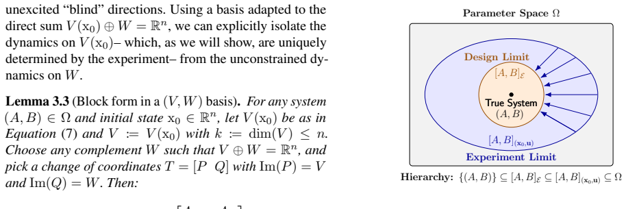
We show that the experimental setup, i.e., the realized initial state and control input, dictates a fundamental limit on the information recoverable from the observed trajectory. We develop a geometric characterization of this limit and derive a closed-form description of all systems consistent with the experimental setup. Crucially, we prove that even when the full system is not identifiable, the restricted dynamics on the subspace reachable by the experiment remain uniquely determined.

What carries the argument

The reachable subspace determined by the initial state and input sequence, which carries the uniquely identifiable restricted dynamics of the LTI system.

If this is right

Model fitting algorithms must account for non-uniqueness outside the reachable subspace to avoid spurious conclusions.
Predictions and control actions based on learned models are reliable only within the experimentally reachable region.
The closed-form description of consistent systems enables explicit enumeration of possible dynamics matching the data.
Standard identifiability conditions such as controllability are not required for unique recovery of the restricted dynamics.

Where Pith is reading between the lines

These are editorial extensions of the paper, not claims the author makes directly.

Experiment designers could prioritize inputs that enlarge the reachable subspace to recover more of the system.
Partial identifiability results like this may extend to nonlinear systems by linearizing around operating points.
In applications like robotics or biology, focusing learning on the reachable subspace could improve robustness when full excitation is impractical.

Load-bearing premise

The system is linear time-invariant and all observations come from one finite trajectory under a fixed initial condition and input sequence.

What would settle it

Finding two distinct linear systems that agree on the reachable subspace dynamics but produce different trajectories for the same initial state and inputs, or a single trajectory where multiple different restricted dynamics fit the data equally well.

Figures

Figures reproduced from arXiv: 2605.12010 by Ayb\"uke Ulusarslan, Niki Kilbertus, Nora Schneider.

**Figure 1.** Figure 1: Non-identifiability from a single realized experiment. Two distinct LTI-systems are indistinguishable from the observed experiment (left), but they yield different trajectories under a new experimental condition (right). 2 PROBLEM STATEMENT Problem Setting. We consider the inverse problem of identifying the parameters of an unknown, continuous-time linear time-invariant (LTI) system from observed state-i… view at source ↗

**Figure 2.** Figure 2: Partial vs. Full Identifiability of a Threedimensional System. (Left) The realized trajectory stays in a proper visible subspace (blue), so only the dynamics induced on that subspace are identifiable (i.e., this restriction represents the identifiable subsystem); dynamics on the complement (gray) are unconstrained by the experiment. (Right) The visible subspace spans the entire state space, and thus the … view at source ↗

**Figure 3.** Figure 3: Hierarchy of system uncertainty sets for a fixed initial state x0. Experiment-consistent set [A, B]e can be larger than the design-consistent set [A, B]E , but collapses to it under trajectory informativeness. form an orthonormal basis for V (x0). We define the minimal coordinates ξ(t) ∈ R k via the projection ξ(t) := P ⊤ V x(t). Define the joint regressor z(t) := [ξ(t) ⊤, u(t) ⊤] ⊤ ∈ R k+m. A realized tra… view at source ↗

**Figure 4.** Figure 4: Identifiability in sparse LTI systems. Fraction of controllable systems (A, B) under varying densities (x-axis) and state dimensions (y-axis). px0 0.25 0.50 0.75 1.0 τx0 0.27 0.52 0.76 1.00 [PITH_FULL_IMAGE:figures/full_fig_p006_4.png] view at source ↗

**Figure 5.** Figure 5: Estimation error in full state space vs. visible subspace. Comparison of the relative estimation error for the full system and the restriction to the visible subspace across four identification methods (DMDc, MOESP, SINDy, and NODE) for a system with dimensionality n = 10. (Top) Errors for increasing Gaussian observation noise levels σ ∈ {0, 10−3 , 10−2 , 10−1 , 0.5}. (Bottom) Errors for visibility dimensi… view at source ↗

**Figure 6.** Figure 6: Relative estimation error as a function of the sampling step ∆t. Varying the state dimension ( [PITH_FULL_IMAGE:figures/full_fig_p019_6.png] view at source ↗

**Figure 7.** Figure 7: Relative estimation error as a function of the state dimension n at fixed visible subspace dimension k = 5. 19 [PITH_FULL_IMAGE:figures/full_fig_p019_7.png] view at source ↗

**Figure 8.** Figure 8: Data-driven recovery of the visible subspace and subsystem. Systems are drawn from the same construction as in other results, with n = 20, k = 5, m = 2; the dynamics are simulated for T = 80 steps under additive Gaussian observation noise, with η ∈ {0, 10−3 , 10−2 , 10−1 , 0.5}. Left. Three relative estimation errors: REEfull, REEoracle-vis (projection onto oracle-V (x0), REEemp-vis (projection onto Vˆ est… view at source ↗

read the original abstract

Learning governing dynamics from data is a common goal across the sciences, yet it is only well-posed when the underlying mechanisms are identifiable. In practice, many data-driven methods implicitly assume identifiability; when this assumption fails, estimated models can yield spurious predictions and invalid mechanistic conclusions. Classical identifiability guarantees for controlled linear time-invariant (LTI) systems provide sufficient conditions -- controllability and persistent excitation -- but leave open whether identifiability holds when these conditions fail, and which parts of the system remain identifiable without full identifiability. We show that the experimental setup, i.e., the realized initial state and control input, dictates a fundamental limit on the information recoverable from the observed trajectory. We develop a geometric characterization of this limit and derive a closed-form description of all systems consistent with the experimental setup. Crucially, we prove that even when the full system is not identifiable, the restricted dynamics on the subspace reachable by the experiment remain uniquely determined.

Editorial analysis

A structured set of objections, weighed in public.

Desk editor's note, referee report, simulated authors' rebuttal, and a circularity audit. Tearing a paper down is the easy half of reading it; the pith above is the substance, this is the friction.

Desk Editor's Note private letter to a colleague

The paper shows reachable-subspace dynamics are uniquely fixed by a single trajectory even when the full LTI system is not identifiable.

read the letter

The main thing to know is that the authors give a geometric description of all systems consistent with one finite trajectory and prove that the dynamics restricted to the reachable subspace stay uniquely determined even if A and B themselves are not. This is a direct extension of classical controllability results into the partial-excitation regime, with a closed-form characterization of the ambiguity set. That part is new and cleanly stated in the abstract. The work is useful because it replaces vague statements about non-identifiability with an explicit picture of what can still be recovered. The linear-algebra framing makes the limits of a given experiment transparent. The central claim about uniqueness on the reachable part is the piece that could matter for downstream control or prediction tasks. The result sits on standard LTI assumptions and full-state observations from one trajectory, which is a real but narrow scope. The stress-test concern about A-B trade-offs when visited states and inputs are linearly dependent is worth checking against the proofs; the abstract asserts the restricted dynamics are pinned down anyway, so the paper must show that any kernel element leaves the action on the reachable subspace unchanged. Without the derivations in front of me it is hard to judge how tightly that is handled. This is for people working on theoretical system identification and data-driven control who need precise identifiability guarantees rather than generic consistency results. A reader already thinking about partial controllability or experiment design will find the geometric view immediately usable. It deserves a serious referee because the question is fundamental in the subfield and the approach is self-contained. I would send it to review; the core geometric claim is worth verifying even if the proofs need tightening.

Referee Report

1 major / 0 minor

Summary. The paper claims that for controlled linear time-invariant systems observed along a single finite trajectory, the experimental setup (initial state and input sequence) imposes fundamental limits on identifiability. It develops a geometric characterization of the reachable subspace and derives a closed-form description of all consistent (A, B) pairs; crucially, it proves that the induced dynamics restricted to this subspace remain uniquely determined even when the full system is not identifiable.

Significance. If the uniqueness result holds, the work supplies a precise, non-asymptotic account of partial identifiability for LTI systems without requiring controllability or persistent excitation. The closed-form characterization of consistent systems is a concrete strength that could directly inform experiment design and model validation in data-driven control.

major comments (1)

[Proof of uniqueness of restricted dynamics (main theorem)] The central uniqueness claim for the restricted dynamics on the reachable subspace S must explicitly rule out nontrivial kernel elements of the map [A B] that act nontrivially on S. The linear dependence case (constant u_t with x_t proportional across t) produces a kernel containing nonzero delta A supported on S; the geometric argument and closed-form description therefore need to demonstrate that no such element survives the consistency conditions for the observed trajectory.

Simulated Author's Rebuttal

1 responses · 0 unresolved

We thank the referee for their careful reading of the manuscript and for the constructive suggestion regarding the uniqueness proof. We address the major comment below and will revise the manuscript accordingly to strengthen the exposition.

read point-by-point responses

Referee: The central uniqueness claim for the restricted dynamics on the reachable subspace S must explicitly rule out nontrivial kernel elements of the map [A B] that act nontrivially on S. The linear dependence case (constant u_t with x_t proportional across t) produces a kernel containing nonzero delta A supported on S; the geometric argument and closed-form description therefore need to demonstrate that no such element survives the consistency conditions for the observed trajectory.

Authors: We appreciate the referee highlighting the importance of explicitly addressing potential kernel elements of the map [A B] in the uniqueness argument. The reachable subspace S is defined geometrically as the smallest subspace containing the initial state and all states generated by the input sequence along the observed trajectory. The closed-form characterization of consistent (A, B) pairs is obtained by solving the system of linear equations x_{t+1} = A x_t + B u_t for the observed data. Any candidate perturbation (ΔA, ΔB) must satisfy ΔA x_t + ΔB u_t = 0 for every t in the trajectory to remain consistent. Because S is spanned by the observed states and is minimal with respect to the experiment, any nonzero action of ΔA on S would produce a mismatch with the observed next state unless the perturbation is identically zero on S. In the specific linear-dependence case (constant u_t with proportional x_t), the subspace S reduces to a low-dimensional span (often one-dimensional), and the consistency equations collapse to a scalar relation that uniquely fixes the restricted dynamics on S; a nonzero ΔA supported on S would violate this scalar equality. To make the argument fully explicit, we will insert a short lemma immediately preceding the main uniqueness theorem that directly shows no nontrivial kernel element of [A B] can act nontrivially on S while preserving consistency with the observed trajectory. This addition will clarify the geometric and algebraic reasons why such elements are ruled out. revision: yes

Circularity Check

0 steps flagged

No circularity: derivation is self-contained linear-algebraic analysis

full rationale

The paper's central result—that the restricted dynamics on the experiment-reachable subspace remain uniquely determined even without full identifiability—follows directly from the consistency equations A x_t + B u_t = x_{t+1} applied to the observed trajectory, together with a geometric decomposition of the state space. No step reduces by construction to a fitted parameter, a self-referential definition, or a load-bearing self-citation whose content is merely renamed. The closed-form description of consistent systems is obtained by solving the underdetermined linear system whose kernel is characterized explicitly; uniqueness on the reachable subspace is shown by proving that any two solutions agree when restricted to that subspace. This is standard linear-algebra reasoning with no tautological reduction to the inputs.

Axiom & Free-Parameter Ledger

0 free parameters · 2 axioms · 0 invented entities

The work rests on standard linear algebra and control theory assumptions with no free parameters, invented entities, or ad-hoc axioms introduced.

axioms (2)

domain assumption The system is linear time-invariant.
Invoked throughout the abstract as the class of systems under study.
domain assumption Data is generated from a single finite trajectory under fixed initial state and input sequence.
Defines the experimental setup whose limits are characterized.

pith-pipeline@v0.9.0 · 5464 in / 1135 out tokens · 50167 ms · 2026-05-13T06:56:22.293783+00:00 · methodology

discussion (0)

Reference graph

Works this paper leans on

39 extracted references · 39 canonical work pages · 1 internal anchor

[1]

Bellman and K.J

R. Bellman and K.J. Åström. On structural identi- fiability.Mathematical Biosciences, 7(3):329–339,

work page
[2]

Bellman and K

ISSN 0025-5564. doi: https://doi.org/ 10.1016/0025-5564(70)90132-X. URL https: //www.sciencedirect.com/science/ article/pii/002555647090132X

work page doi:10.1016/0025-5564(70)90132-x
[3]

University of Newcastle, 1995

Julio Hernán Braslavsky et al.Frequency domain analysis of sampled-data control systems. University of Newcastle, 1995

work page 1995
[4]

Discovering governing equations from data by sparse identification of nonlinear dynamical systems

Steven L Brunton, Joshua L Proctor, and J Nathan Kutz. Discovering governing equations from data by sparse identification of nonlinear dynamical systems. Proceedings of the national academy of sciences, 113 (15):3932–3937, 2016

work page 2016
[5]

Identifiability Challenges in Sparse Linear Ordinary Differential Equations

Cecilia Casolo, Sören Becker, and Niki Kilbertus. Identifiability challenges in sparse linear ordinary dif- ferential equations, 2025. URL https://arxiv. org/abs/2506.09816

work page internal anchor Pith review Pith/arXiv arXiv 2025
[6]

Neural ordinary differential equations.Advances in neural information processing systems, 31, 2018

Ricky TQ Chen, Yulia Rubanova, Jesse Bettencourt, and David K Duvenaud. Neural ordinary differential equations.Advances in neural information processing systems, 31, 2018

work page 2018
[7]

Springer Science & Business Media, 2012

Tongwen Chen and Bruce A Francis.Optimal sampled- data control systems. Springer Science & Business Media, 2012

work page 2012
[8]

John Wiley & Sons, 1999

Gerald B Folland.Real analysis: modern techniques and their applications. John Wiley & Sons, 1999

work page 1999
[9]

Hagiwara

T. Hagiwara. Preservation of reachability and observ- ability under sampling with a first-order hold.IEEE Transactions on Automatic Control, 40(1):104–107,

work page
[10]

doi: 10.1109/9.362892

work page doi:10.1109/9.362892
[11]

Gra- dient descent learns linear dynamical systems.Journal of Machine Learning Research, 19(29):1–44, 2018

Moritz Hardt, Tengyu Ma, and Benjamin Recht. Gra- dient descent learns linear dynamical systems.Journal of Machine Learning Research, 19(29):1–44, 2018

work page 2018
[12]

SIAM, 2008

Nicholas J Higham.Functions of matrices: theory and computation. SIAM, 2008

work page 2008
[13]

I. W. Jamaludin, N. A. Wahab, N. S. Khalid, S Sahlan, Z. Ibrahim, and M F. Rahmat. N4sid and moesp sub- space identification methods. In2013 IEEE 9th In- ternational Colloquium on Signal Processing and its Applications, pages 140–145, 2013. doi: 10.1109/ CSPA.2013.6530030

work page arXiv 2013
[14]

Mathematical description of linear dynamical systems.Journal of the Society for Industrial and Applied Mathematics, Series A: Control, 1(2):152–192, 1963

Rudolf Emil Kalman. Mathematical description of linear dynamical systems.Journal of the Society for Industrial and Applied Mathematics, Series A: Control, 1(2):152–192, 1963

work page 1963
[15]

On sampling without loss of observability/controllability.IEEE Transactions on Automatic Control, 44(5):1021–1025, 2002

Gerhard Kreisselmeier. On sampling without loss of observability/controllability.IEEE Transactions on Automatic Control, 44(5):1021–1025, 2002

work page 2002
[16]

WCB/McGraw Hill New York, 1998

Robert C Nelson et al.Flight stability and automatic control, volume 2. WCB/McGraw Hill New York, 1998

work page 1998
[17]

Covid-19: A multiwave sir-based model for learning waves.Production and Operations Management, 32(5):1471–1489, 2023

Georgia Perakis, Divya Singhvi, Omar Skali Lami, and Leann Thayaparan. Covid-19: A multiwave sir-based model for learning waves.Production and Operations Management, 32(5):1471–1489, 2023

work page 2023
[18]

Proctor, Steven L

Joshua L. Proctor, Steven L. Brunton, and J. Nathan Kutz. Dynamic mode decomposition with control. SIAM Journal on Applied Dynamical Systems, 15(1): 142–161, 2016. doi: 10.1137/15M1013857. URL https://doi.org/10.1137/15M1013857

work page doi:10.1137/15m1013857 2016
[19]

Identifiability analysis of linear ordinary differen- tial equation systems with a single trajectory.Applied Mathematics and Computation, 430:127260, 2022

Xing Qiu, Tao Xu, Babak Soltanalizadeh, and Hulin Wu. Identifiability analysis of linear ordinary differen- tial equation systems with a single trajectory.Applied Mathematics and Computation, 430:127260, 2022

work page 2022
[20]

An interven- tional perspective on identifiability in gaussian lti sys- tems with independent component analysis

Goutham Rajendran, Patrik Reizinger, Wieland Bren- del, and Pradeep Kumar Ravikumar. An interven- tional perspective on identifiability in gaussian lti sys- tems with independent component analysis. InCausal Learning and Reasoning, pages 41–70. PMLR, 2024

work page 2024
[21]

A persistency of excitation condition for continuous-time systems.IEEE Control Systems Letters, 7:589–594, 2022

Paolo Rapisarda, M Kanat Camlibel, and HJ Van Waarde. A persistency of excitation condition for continuous-time systems.IEEE Control Systems Letters, 7:589–594, 2022

work page 2022
[22]

Near optimal finite time identification of arbitrary linear dynamical systems

Tuhin Sarkar and Alexander Rakhlin. Near optimal finite time identification of arbitrary linear dynamical systems. InInternational Conference on Machine Learning, pages 5610–5618. PMLR, 2019

work page 2019
[23]

Persistency of exci- tation in continuous-time systems.Systems & control letters, 9(3):225–233, 1987

Nahum Shimkin and Arie Feuer. Persistency of exci- tation in continuous-time systems.Systems & control letters, 9(3):225–233, 1987

work page 1987
[24]

Learning without mix- ing: Towards a sharp analysis of linear system identi- fication

Max Simchowitz, Horia Mania, Stephen Tu, Michael I Jordan, and Benjamin Recht. Learning without mix- ing: Towards a sharp analysis of linear system identi- fication. InConference On Learning Theory, pages 439–473. PMLR, 2018

work page 2018
[25]

Uncovering differential equations from data with hidden variables.Physical Review E, 105(5):054209, 2022

Agustín Somacal, Yamila Barrera, Leonardo Boechi, Matthieu Jonckheere, Vincent Lefieux, Dominique Pi- card, and Ezequiel Smucler. Uncovering differential equations from data with hidden variables.Physical Review E, 105(5):054209, 2022. 9

work page 2022
[26]

Springer Science & Business Media, 2013

Eduardo D Sontag.Mathematical control theory: deterministic finite dimensional systems, volume 6. Springer Science & Business Media, 2013

work page 2013
[27]

Identifiability of linear and linear-in- parameters dynamical systems from a single trajectory

Shelby Stanhope, Jonathan E Rubin, and David Swigon. Identifiability of linear and linear-in- parameters dynamical systems from a single trajectory. SIAM Journal on Applied Dynamical Systems, 13(4): 1792–1815, 2014

work page 2014
[28]

Identifiability analysis of lin- ear ode systems with hidden confounders.Advances in Neural Information Processing Systems, 37:59054– 59092, 2024

Yuanyuan Wang, Biwei Huang, Wei Huang, Xi Geng, and Mingming Gong. Identifiability analysis of lin- ear ode systems with hidden confounders.Advances in Neural Information Processing Systems, 37:59054– 59092, 2024

work page 2024
[29]

A note on persistency of excitation

Jan C Willems, Paolo Rapisarda, Ivan Markovsky, and Bart LM De Moor. A note on persistency of excitation. Systems & Control Letters, 54(4):325–329, 2005

work page 2005
[30]

Springer, 1974

Walter Murray Wonham.Linear multivariable control, volume 101. Springer, 1974

work page 1974
[31]

On controllability and persistency of excitation in data- driven control: Extensions of willems’ fundamental lemma

Yue Yu, Shahriar Talebi, Henk J Van Waarde, Ufuk Topcu, Mehran Mesbahi, and Behçet Açıkmes, e. On controllability and persistency of excitation in data- driven control: Extensions of willems’ fundamental lemma. In2021 60th IEEE Conference on Decision and Control (CDC), pages 6485–6490. IEEE, 2021. 10 Limits of Learning Linear Dynamics from Experiments (Su...

work page 2021
[32]

Furthermore, multiplying any vector in V(x 0) by A yields a linear combination of terms up to An[x0 B]

V(x 0) satisfies the conditions.By the definition of the Krylov sequence, the 0−th order terms include x0 and the columns of B, meaning {x0} ∪Im(B)⊆V(x 0). Furthermore, multiplying any vector in V(x 0) by A yields a linear combination of terms up to An[x0 B]. By the Cayley-Hamilton theorem, An can be expressed as a linear combination of lower powers A0, ....

work page
[33]

Because x0 ∈S and S is A−invariant, we necessarily have Akx0 ∈S for all k∈ {0,

Minimality.Let S⊆R n be any arbitrary A−invariant subspace (AS⊆S ) that contains {x0} ∪Im(B) . Because x0 ∈S and S is A−invariant, we necessarily have Akx0 ∈S for all k∈ {0, . . . , n−1} . By the same logic, because Im(B)⊆S , we have AkIm(B)⊆S for all k∈ {0, . . . , n−1} . Because S is a linear subspace, it is closed under vector addition and scalar multi...

work page
[34]

By definition of [A, B]E, the trajectories agree for every admissible input u∈ U

Necessity ("=⇒"): Assume that ( ˜A, ˜B)∈[A, B] E. By definition of [A, B]E, the trajectories agree for every admissible input u∈ U . In particular, since the zero input is admissible via Assumption 2.2, we may choose u(·)≡0 m and obtain equality of the autonomous responses: ∀t∈[0, T] :e Atx0 =e ˜Atx0. Since both sides are real-analytic int, we get ∀k∈N 0 ...

work page
[35]

Since ˜A V(x 0) =A| V(x 0), andV(x 0)isA−invariant(*), it is also ˜A−invariant: ∀v∈V: ˜Av=Av (*) ∈V⇐ ⇒ ˜AV⊆V def

Sufficiency ("⇐="): Let ( ˜A, ˜B) be any block matrix in Rn×(n+m) such that ˜A V(x 0) =A| V(x 0) and ˜B=B . Since ˜A V(x 0) =A| V(x 0), andV(x 0)isA−invariant(*), it is also ˜A−invariant: ∀v∈V: ˜Av=Av (*) ∈V⇐ ⇒ ˜AV⊆V def. ⇐ ⇒Vis ˜A−invariant. All powers agree onV(x 0). Next, we argue that all powers agree onV(x 0): ∀k∈N 0 : ˜Ak V(x 0) =A k V(x 0) . This f...

work page
[36]

To show: ( ˜A, ˜B)∈[A, B] (x0,u) =⇒( ˜A, ˜B)∈[A, B] E ← →˜φ=φ=⇒ ˜A V(x 0) =A V(x 0) ∧ ˜B=B

Reverse Inclusion ( [A, B](x0,u) ⊆[A, B] E):Let ( ˜A, ˜B)∈[A, B] (x0,u) and shorten system responses as φ:= φ([0, T]|A, B,x 0,u)and˜φ:= ˜φ([0, T]| ˜A, ˜B,x 0,u). To show: ( ˜A, ˜B)∈[A, B] (x0,u) =⇒( ˜A, ˜B)∈[A, B] E ← →˜φ=φ=⇒ ˜A V(x 0) =A V(x 0) ∧ ˜B=B. 16 Since˜φ=φ, the time derivatives on[0, T]must match as well: ∀t∈[0, T] : ˜Ax(t) + ˜Bu(t) =Ax(t) +Bu(t...

work page
[37]

Reachable space is preserved.From span{Ak dBd} ⊆span{A kBd} with w=B d, span{Ak dBd} ⊆span{A kBd}. If ∆t is nonpathological on thereachable spectrum σr(A, B), then g(λ)̸= 0 for all λ∈σ r(A, B), so g(A) is invertible on Rct 0 := span{AkB}and span{AkBd}= span{A kg(A)B}= span{A kB}=R ct 0 , givingR dt 0 ⊆ R ct 0 . For the reverse inclusion, restrict attentio...

work page
[38]

For the reverse inclusion on theautonomouspart Kn(A, x0), assume λ7→e λ∆t is injective on all of σ(A)

Visible subspace is preserved.From span{Ak dBd} ⊆span{A kBd} with w∈ {x 0} ∪col(B) and Bd =g(A)B we get the easy directionV dt(x0)⊆V ct(x0). For the reverse inclusion on theautonomouspart Kn(A, x0), assume λ7→e λ∆t is injective on all of σ(A). By the same analytic/Jordan-block argument as above (now on the full space), for each polynomialp there is a q wi...

work page
[39]

good”),x (b) 0 =   1 −1 0   (“bad

Informativeness under ZOH.To bridge the continuous-time informativeness to ZOH inputs, we rely on the exact discrete-time dynamics on the visible subspaceV(x 0): ξ[j+ 1] =A d,V ξ[j] +B d,V u[j], where Ad,V =e AV ∆t and Bd,V = R ∆t 0 eAV sBV ds. By Step 3, if ∆t is non-pathological, (Ad,V ,[x 0 Bd,V ]) is a controllable pair onR n (wherek= dim(V(x 0))). Fo...

work page