Fluctuation-Dissipation Framework for Size-Dependent Surface Tension

Pressure derivatives of raw and central moments It is convenient to begin with the pressure derivative of lnQ: ∂lnQ ∂P T,N = 1 Q ∂Q ∂P T,N = 1 Q Z ∞ 0 dV ∑ k (−βV)exp −β PV+E k(V;N) =−β⟨V⟩=−β ν 1. (A4) Differentiating once more yields ∂ 2 lnQ ∂P 2 T,N =−β ∂ ν1 ∂P T,N =β 2 h ⟨V2⟩ −(⟨V⟩) 2 i =β 2m2, (A5) wherem 2 is the second central moment, i.e., the vari...

1 ν1 ∂m 2 ∂P T,N − m2 ν2 1 ∂ ν1 ∂P T,N # = 1 (kBT) 2

Compressibility and its pressure derivative The isothermal compressibility is defined as βT (T,P) =− 1 ν1 ∂ ν1 ∂P T,N .(A13) Using Eq. (A8), we obtain the standard fluctuation formula βT (T,P) = 1 kBT m2 ν1 ,(A14) which coincides with Eq. (14) in the main text. 14 Differentiating Eq. (A14) with respect to pressure gives β ′ T (T,P) = ∂ βT ∂P T,N = 1 kBT "...

Fluctuation–response identity for the planar-limit relation Equations (A12) imply a compact identity for the pres- sure response of the relative width of the volume distribution. Writingσ V = √m2 and using ln(σV /ν1) = 1 2 lnm 2 −lnν 1, we obtain ∂ ∂P T,N ln σV ν1 = 1 2m2 ∂m 2 ∂P T,N − 1 ν1 ∂ ν1 ∂P T,N =β m2 ν1 − m3 2m2 .(A16) Equivalently, 1 2kBT 2 m2 ν1...

Coexistence reference state and local notation Throughout this Appendix, temperatureTis fixed and the reference state is the planar liquid–vapor coexistence point (T,P0), where P0 =P sat(T),µ l(T,P0) =µ v(T,P0).(B1) For each phasei∈ {l,v}, we write ρi0 ≡ρ i(T,P0),∆P i ≡Pi −P0,∆ρ i ≡ ρi −ρ i0 ρi0 .(B2) Unless stated otherwise, all pressure derivatives in t...

These pressure derivatives provide the local expansion co- efficients used later when the chemical-potential equality is expanded directly in excess-pressure variables

Pressure derivatives of the chemical potential Along an isotherm, the chemical potential satisfies the stan- dard relation ∂ µi ∂P T = 1 ρi .(B5) Using ∂ ρi ∂P T =β T,iρi,(B6) the second pressure derivative becomes ∂ 2µi ∂P 2 T =− βT,i ρi .(B7) Differentiating once more gives ∂ 3µi ∂P 3 T = β 2 T,i −β ′ T,i ρi .(B8) 15 Evaluated at the coexistence referen...

(B10) Using Eq

Local pressure expansion of the chemical potential Expandingµ i(T,P)aboutP=P 0 gives µi(P0 +∆Pi) =µ i(P0) +µ ′ i,0∆Pi + 1 2 µ ′′ i,0∆P2 i + 1 6 µ ′′′ i,0∆P3 i +O(∆P 4 i ). (B10) Using Eq. (B9), this becomes µi(P0 +∆Pi) =µ i(P0) + ∆Pi ρi0 − βT,i 2ρi0 ∆P2 i + β 2 T,i −β ′ T,i 6ρi0 ∆P3 i +O(∆P 4 i ). (B11) Equation (B11) is the local pressure expansion used ...

Us- ing the chain rule together with Eqs

Density derivatives of the chemical potential We next construct the local density representation ofµi. Us- ing the chain rule together with Eqs. (B5) and (B6), we obtain ∂ µi ∂ ρi T = ∂ µi ∂P T ∂ ρi ∂P T = 1 βT,iρ2 i .(B12) Differentiating with respect toρ i at fixedTgives ∂ 2µi ∂ ρ2 i T =− 2+β ′ T,i/β 2 T,i βT,iρ3 i .(B13) Equivalently, using Eq. (B4), ∂...

(B17) Using Eq

Local density expansion of the chemical potential Writing ρi =ρ i0(1+∆ρ i),(B16) we expandµ i(ρi;T)aboutρ i0: µi ρi0(1+∆ρ i) =µ i(ρi0) + ∂ µi ∂ ρi T ρi0 ρi0∆ρi + 1 2 ∂ 2µi ∂ ρ2 i T ρi0 ρ2 i0∆ρ2 i +O(∆ρ 3 i ). (B17) Using Eq. (B15), we obtain µi ρi0(1+∆ρ i) =µ i(ρi0) + ∆ρi βT,iρi0 − 1 2βT,iρi0 2+ β ′ T,i β 2 T,i ! ∆ρ2 i +O(∆ρ 3 i ) =µ i(ρi0) + ∆ρi βT,iρi0 ...

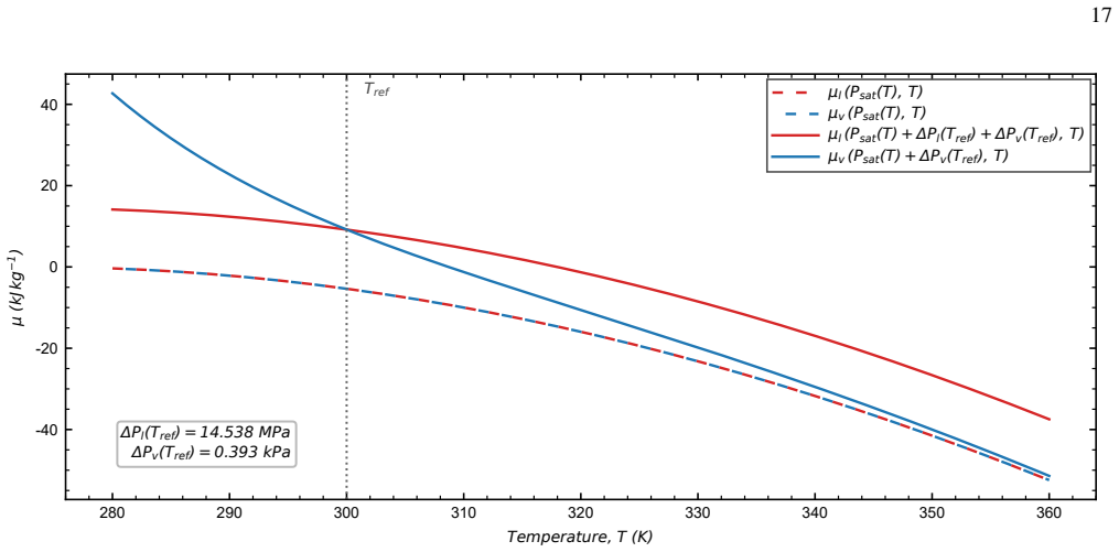
Figure 3 contrasts the planar coexistence branches with the branches evaluated at the shifted liquid and vapor pressures corresponding to a representative curved droplet

Illustrative coexistence and shifted-pressure chemical-potential branches Although the present Appendix is devoted to local one- phase expansions, it is useful to visualize the chemical- potential branches that later enter the capillary–chemical bal- ance through shifted pressure arguments. Figure 3 contrasts the planar coexistence branches with the branc...

Role in the later appendices The results of the present Appendix serve only as local one- phase input for the later derivations. Equation (B11) supplies the one-phase pressure expansion of the chemical potential used in Appendix D, where the same capillary–chemical bal- ance is expanded in excess-pressure variables. Equation (B18) supplies the one-phase d...

(C3) For later convenience, we introduce the compact combination Ai ≡1+ β ′ i β 2 i .(C4) At the present stage, all relations are purely one-phase and local

Reference state and one-phase variables Throughout this Appendix, temperatureTis fixed and the reference state is the planar liquid–vapor coexistence point (T,P0), where P0 =P sat(T),µ l(T,P0) =µ v(T,P0).(C1) For each phasei∈ {l,v}, we define ρi0 ≡ρ i(T,P0),∆P i ≡Pi −P0,∆ρ i ≡ ρi −ρ i0 ρi0 .(C2) We also write βi ≡β T,i(T,P0), β ′ i ≡ ∂ βT,i ∂P T P0 , β ′′...

Forward one-phase series:∆P i(∆ρi) We begin from the local thermal equation of state of phase i, written along an isotherm asP i =P i(ρ;T). The one-phase excess pressure is then ∆Pi =P i ρi0(1+∆ρ i);T −Pi(ρi0;T).(C5) Along an isotherm, the standard identities ∂ µi ∂P T = 1 ρi , ∂ ρi ∂P T =β T,i(T,P)ρ i (C6) imply ∂P ∂ ρi T = 1 βT,i(T,P)ρ i .(C7) Evaluatin...

(C12) to the order required later in the manuscript

Local inverse series:∆ρ i(∆Pi) We next invert Eq. (C12) to the order required later in the manuscript. We seek a local inverse relation of the form ∆ρi =a 1∆Pi +a 2∆P2 i +O(∆P 3 i ).(C13) Substituting Eq. (C13) into Eq. (C12) and matching equal powers of∆P i, we obtain a1 =β i,a 2 = 1 2 1+ β ′ i β 2 i β 2 i = 1 2 Aiβ 2 i .(C14) Therefore, ∆ρi =β i∆Pi + 1 ...

For the water regime emphasized in the 18 manuscript, it is therefore useful to support that these retained orders remain adequate over the interval of practical interest

Water-based support for the retained local truncation orders The one-phase local series derived above are used later only at low retained orders. For the water regime emphasized in the 18 manuscript, it is therefore useful to support that these retained orders remain adequate over the interval of practical interest. The present subsection serves exactly t...

Equation (C12) provides the forward one-phase thermal-equation-of-state series, whereas Eqs

Use in the later derivations The results of the present Appendix are used later only as local one-phase input. Equation (C12) provides the forward one-phase thermal-equation-of-state series, whereas Eqs. (C15) and (C17) provide the corresponding local inverse series. In the later density-based derivation, these inverse one- phase relations are combined wi...

II A, this corre- sponds to a liquid droplet or liquid filament surrounded by vapor, so that the liquid pressure exceeds the vapor pressure by the Laplace amount

Pressure-side setup and shifted arguments Throughout this Appendix, temperatureTis fixed and the reference state is the planar coexistence point(T,P 0), where P0 =P sat(T),µ l(T,P0) =µ v(T,P0).(D1) We define the phase excess pressures and the capillary pres- sure difference by ∆Pv ≡P v −P0,∆P l ≡P l −P0,∆P≡P l −Pv,(D2) so that ∆Pl =∆P v +∆P.(D3) With the ...

Local pressure-expanded capillary–chemical balance At fixedT, the pressure derivatives of the chemical poten- tial satisfy ∂ µi ∂P T = 1 ρi , ∂ 2µi ∂P 2 T =− βT,i ρi , ∂ 3µi ∂P 3 T = β 2 T,i −β ′ T,i ρi . (D8) 19 10 20 30 40 50 60 70R (nm) -1.1 -1.0 -0.9 -0.8 -0.7 -0.6 -0.5 -0.4 δ (Å) 0 5 10 15 20 25 30 35 a 10 20 30 40 50 60 70R (nm) -1.1 -1.0 -0.9 -0.8 ...

Accordingly, the planar-limit coefficient is not obtained from a prior separate pressure-only symbolic balance

Minimal pressure-side formulation We now combine the local pressure-expanded balance with the Tolman-corrected capillary relation ∆P=Hγ ∞ 1−Hδ Tolman .(D11) A point that matters for interpretation is that, in the actual symbolic workflow, the first retained mixed pressure-side rela- tion already contains explicitΠ v-dependence, because the liq- uid branch...

At this level, ex- plicit supersaturation dependence is already present, because the liquid-side bivariate expansion generates mixed terms con- taining both∆P v and∆P

First retained pressure-side Tolman-sensitive relation We next retain the first mixed pressure-side structure pro- duced directly by the symbolic workflow. At this level, ex- plicit supersaturation dependence is already present, because the liquid-side bivariate expansion generates mixed terms con- taining both∆P v and∆P. After substitution of Eq. (D11) i...

Including the next retained supersaturation-dependent terms If one retains the nextΠ 2 v-level contributions in the pressure-side algebra, the mixed balance acquires both quadratic vapor-response terms and higher liquid-side mixed terms. At this level, the Tolman-sensitive relation may still be written in compact form as ∆= Np(Πv) Dp(Πv) ,(D23) 21 with Np...

Practical scope of the pressure-side formulation The pressure-side formulation developed here is one legit- imate local formulation of the same capillary–chemical bal- ance used in the main text. Its main value is structural: it gives a direct pressure-side view of the leading supersaturation rela- tion, the planar-limit coefficient obtained within the mi...

II A, this corre- sponds to a liquid droplet or liquid filament surrounded by vapor, so that the liquid pressure exceeds the vapor pressure by the Laplace amount

Density-side setup and adopted retained ordering Throughout this Appendix, temperatureTis fixed and the reference state is the planar coexistence point(T,P 0), where P0 =P sat(T),µ l(T,P0) =µ v(T,P0).(E1) We use the same excess-pressure variables as in the main text and in Appendix D: ∆Pv ≡P v −P0,∆P l ≡P l −P0,∆P≡P l −Pv,(E2) so that ∆Pl =∆P v +∆P.(E3) W...

Leading two-phase density coupling from chemical-potential equality The local density-side expansion of the chemical potential obtained in Appendix B gives, for each phasei∈ {l,v}, µi ρi0(1+∆ρ i) =µ i(ρi0) + ∆ρi βT,iρi0 +O(∆ρ 2 i ).(E6) Imposing chemical equilibrium, µl =µ v,(E7) and using Eq. (E1), we obtain at leading order ∆ρl βT,l ρl0 − ∆ρv βT,vρv0 =0...

One-phase liquid and vapor re-expansions used in the adopted derivation From Appendix C, the one-phase inverse excess-pressure / relative-density series gives, for the liquid branch, ∆ρl =β T,l ∆Pl + 1 2 1+ β ′ T,l β 2 T,l ! (βT,l ∆Pl)2 +O(∆P 3 l ).(E10) For compactness, we define Al ≡1+ β ′ T,l β 2 T,l ,(E11) so that Eq. (E10) becomes ∆ρl =β T,l ∆Pl + 1 ...

(E12) into the leading density cou- pling (E9) gives ∆ρv = βT,vρv0 ρl0 ∆Pl + 1 2 Al βT,vβT,l ρv0 ρl0 ∆P2 l +O(∆P 3 l )

Reduced excess-pressure balance of the adopted density-based formulation Substituting Eq. (E12) into the leading density cou- pling (E9) gives ∆ρv = βT,vρv0 ρl0 ∆Pl + 1 2 Al βT,vβT,l ρv0 ρl0 ∆P2 l +O(∆P 3 l ). (E14) Equating this with the retained vapor-side relation (E13) and dividing byβ T,v, we obtain ∆Pv ρl0 ρv0 =∆P l + 1 2 Al βT,l ∆P2 l +O(∆P 3 l ,∆P...

Mixed finite-curvature balance in(Π v,h,∆) We now combine Eq. (E15) with the Tolman-corrected cap- illary relation ∆Pl −∆Pv =Hγ ∞ 1−Hδ Tolman .(E16) For convenience, we introduce the same dimensionless vari- ables as in Appendix D, rρ ≡ ρv0 ρl0 ,Π v ≡β T,l ∆Pv, h≡Hγ ∞βT,l ,∆≡ δTolman γ ∞βT,l . (E17) Equation (E16) then implies βT,l ∆Pl =Π v +h(1−h∆).(E18)...

(E19): Πv −2+2r ρ +r ρAlΠv +2hr ρ [1+A lΠv] =0.(E20) This relation is used only as an auxiliary relation controlling the supersaturation

Auxiliary supersaturation control relation The auxiliary supersaturation-control relation is built only from the explicitly retained∆-free terms of orderh 0 andh 1 in Eq. (E19): Πv −2+2r ρ +r ρAlΠv +2hr ρ [1+A lΠv] =0.(E20) This relation is used only as an auxiliary relation controlling the supersaturation. It is not itself the Tolman-sensitive rela- tion...

Tolman-sensitive relation and planar-limit extraction After the auxiliary supersaturation step has fixed the lead- ing scaling ofΠ v, the Tolman contribution is extracted only from the explicitly retainedh 2-sector of Eq. (E19). That sec- tor is Al −2∆−2A lΠv∆=0,(E25) which yields the Tolman-sensitive relation ∆(Πv) = Al 2(1+A lΠv) .(E26) The planar-limit...

Finite-curvature continuation If one keeps Eq. (E26) at finiteΠ v, rather than taking the strict planar limit immediately, one obtains the non-strict finite-curvature continuation ∆cont(Πv) = Al 2(1+A lΠv) .(E29) In dimensional form, δ cont Tolman = δ planar Tolman 1+ βT,l + β ′ T,l βT,l ∆Pv .(E30) This expression reduces to the planar-limit result as∆P v...

Decomposition of the quadratic liquid contribution under composition of local series To understand why comparison variants can yield differ- ent planar coefficients, it is useful to isolate the two distinct quadratic liquid contributions before they are composed. From Appendix B, the local liquid chemical-potential ex- pansion in the relative density devi...

Comparison variants and coefficient migration We now record three comparison variants, distinguished by which quadratic liquid contribution survives in the retained h2-sector after composition. (i) Chemical-potential quadratic contribution only.If one retains only the quadratic contribution originating from the local chemical-potential expansion, the repr...

Recovery of the pressure-side planar coefficient A noteworthy feature of the comparison variants is that the coefficient obtained when both quadratic liquid contributions are retained together, ∆(µ+inv) 0 =− 1 2 ,(E50) recovers the minimal pressure-side planar coefficient derived in the pressure-side formulation of Appendix D. In dimen- sional form, δ (µ+...

Status of the comparison variants The adopted manuscript-level derivation is the one given in Secs. E 1–E 8. Within that derivation, the reported planar-limit result is Eq. (E28). The comparison variants introduced after- ward do not modify that result and are not alternative adopted formulations. Their function is narrower. They document how different re...

Purpose and scope The adopted density-based derivation has already been completed in Appendix E. In particular, the auxiliary supersaturation-control relation is constructed there only from the explicitly retained∆-free terms of ordersh 0 andh 1, whereas the Tolman-sensitive relation is extracted only from the explicitly retained sector of orderh 2. The p...

(F1) Here rρ ≡ ρv0 ρl0 ,Π v ≡β T,l ∆Pv, h≡Hγ ∞βT,l ,∆≡ δTolman γ ∞βT,l , (F2) and Al ≡1+ β ′ T,l β 2 T,l .(F3) For the present diagnostic purpose, it is convenient to sepa- rate Eq

Diagnostic quantities inherited from Appendix E We begin from the retained mixed balance derived in Ap- pendix E, 0=Π v −2+2r ρ +r ρAlΠv +2hr ρ [1+A lΠv] +h 2rρ [Al −2∆−2A lΠv∆]. (F1) Here rρ ≡ ρv0 ρl0 ,Π v ≡β T,l ∆Pv, h≡Hγ ∞βT,l ,∆≡ δTolman γ ∞βT,l , (F2) and Al ≡1+ β ′ T,l β 2 T,l .(F3) For the present diagnostic purpose, it is convenient to sepa- rate ...

Throughout, the coexistence reference state is(T,P 0), withP 0 =P sat(T), and all coefficients entering Eqs

EOS-based evaluation procedure for water To evaluate the hierarchy ratio (F7) for water, we use ther- modynamic properties evaluated from the IAPWS-IF97 in- dustrial formulation as empirical input for the required liq- uid and vapor quantities near coexistence. Throughout, the coexistence reference state is(T,P 0), withP 0 =P sat(T), and all coefficients ...

In representative near-ambient conditions, one finds |R| ∼10 −2–10−1 (F10) for a wide range of nanometric radii and moderate choices of δTolman

Water-specific hierarchy behavior For water away from criticality, and for the nanometric regime emphasized in the manuscript, the EOS-based esti- mates show that the magnitude of the diagnostic ratio (F7) remains typically below unity and, over a broad practically relevant range, substantially below unity. In representative near-ambient conditions, one f...

Practical implication for the adopted density-based formulation For water under the conditions considered in the manuscript, the hierarchy condition|R| ≪1 supports the practical relevance of the adopted density-based formulation developed in Appendix E. More specifically, it supports the strategy in which the auxiliary supersaturation-control rela- tion i...

Interaction models for water in relation to protein hydration,

Limitations The present hierarchy support is intentionally water- specific and regime-specific. It is aimed at the weakly compressible near-coexistence regime emphasized in the manuscript, not at critical or near-spinodal conditions. Near the critical region, the coexistence density contrast de- creases, the compressibilities grow strongly, and both the l...

work page doi:10.1063/1.3376612/16122339/141101_1_online.pdf 2020