Properties of the quantum vacuum in non-abelian gauge theories
Pith reviewed 2026-05-20 09:48 UTC · model grok-4.3
The pith
The mass of the lightest glueball sets the exponential decay of the Casimir energy in non-abelian gauge theories at large boundary separations.
A machine-rendered reading of the paper's core claim, the machinery that carries it, and where it could break.
Core claim
The author computes the Casimir energy non-perturbatively and concludes that, in pure gauge theories, the energy at large separation L decays exponentially with a rate fixed by the mass of the lightest glueball, as expected once the infrared regime is dominated by massive states rather than the massless ultraviolet degrees of freedom.
What carries the argument
Monte Carlo evaluation of the vacuum energy for different boundary conditions, with the lightest glueball mass providing the inverse length scale that governs the exponential suppression at large L.
If this is right
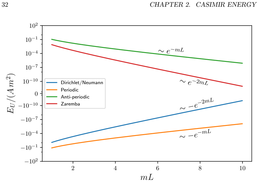
- The Casimir energy interpolates between polynomial decay in the ultraviolet and exponential decay in the infrared.
- The decay constant at large L equals the lightest glueball mass.
- Boundary conditions modify the overall energy but leave the large-L asymptotic form unchanged.
- The infrared spectrum of glueballs directly controls long-distance vacuum properties.
Where Pith is reading between the lines
- Casimir energy simulations could provide an independent route to glueball masses without dedicated spectroscopy runs.
- The same logic might connect vacuum energy between boundaries to confinement scales in other gauge theories.
- Varying the lattice spacing in future runs could separate genuine glueball effects from discretization artifacts.
Load-bearing premise
The non-perturbative infrared regime is dominated by a single massive glueball whose mass alone sets the exponential fall-off of the Casimir energy.
What would settle it
A lattice calculation at large L that measures an exponential decay rate clearly different from the independently computed lightest glueball mass would falsify the claim.
Figures


read the original abstract
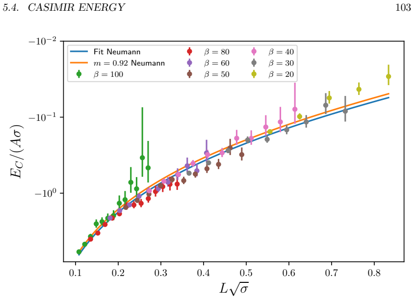
In this thesis we analyze the quantum vacuum properties of non-abelian gauge theories. We calculate the energy of the quantum vacuum by non-perturbative methods using Monte Carlo simulations, focusing on the contribution of boundary effects to the Casimir energy. In particular, we analyze the dependence of the vacuum energy on the types of boundary conditions. The main goal is to clarify the behaviour of this energy for large separation L between the boundaries of the domain where the fields are confined. Usually this Casimir energy decreases polynomially with L for massless theories and exponentially for massive theories. Since gauge theories interpolate between these two regimes, being massless in the ultraviolet regime and massive in the infrared regime, one expects a very special change of behaviour from the perturbative to the non-perturbative approaches. In pure gauge theories there is evidence of the existence of glueball states in the low energy spectrum with a non-vanishing mass, the second goal will be testing if the mass of the lightest glueball is responsible for the exponential decay of the Casimir energy of gauge theories.
Editorial analysis
A structured set of objections, weighed in public.
Referee Report
Summary. The manuscript analyzes the quantum vacuum properties of non-abelian gauge theories by computing the Casimir energy via Monte Carlo simulations on lattices with varying boundary conditions. The central claim is that the exponential decay of this energy at large boundary separation L is set by the mass of the lightest glueball, providing a test of the non-perturbative infrared regime.
Significance. If the central claim is substantiated with adequate controls, the work would furnish direct numerical evidence linking the glueball spectrum to the large-distance fall-off of boundary-induced vacuum energies. This would strengthen the physical picture of glueball dominance in the IR of pure gauge theories and could inform related studies of confinement. The Monte Carlo approach with boundary-condition variation is a reasonable strategy for the problem.
major comments (2)
- [Section 4 (Results)] The extraction of the exponential decay constant from the Casimir energy difference is not described with sufficient detail (no explicit fitting procedure, range of L used, or error analysis is given), making it impossible to verify that the observed fall-off is cleanly due to the lightest glueball rather than boundary artifacts or multi-state contributions.
- [Section 5 (Discussion)] No cross-check is presented between the decay constant fitted from the Casimir energy and an independent glueball mass measurement performed on the identical lattice ensembles and volumes; without this, the identification of the lightest glueball as the source of the exponential remains unverified and load-bearing for the main conclusion.
minor comments (2)
- [Introduction] The abstract states the goals clearly but the manuscript would benefit from an explicit statement of the precise definition of the Casimir energy difference used to cancel UV divergences.
- [Results] Figures displaying energy versus L should include both linear and semi-log scales to make the exponential regime visually apparent.
Simulated Author's Rebuttal
We thank the referee for the careful reading of our manuscript and the constructive comments on the analysis of the Casimir energy in non-abelian gauge theories. The suggestions help clarify the numerical extraction and strengthen the link to the glueball spectrum. We address each major comment below and have updated the manuscript accordingly.
read point-by-point responses
-
Referee: [Section 4 (Results)] The extraction of the exponential decay constant from the Casimir energy difference is not described with sufficient detail (no explicit fitting procedure, range of L used, or error analysis is given), making it impossible to verify that the observed fall-off is cleanly due to the lightest glueball rather than boundary artifacts or multi-state contributions.
Authors: We agree that additional details are required for reproducibility. In the revised Section 4 we now specify the fitting procedure: the Casimir energy difference is fitted to the single-exponential form A exp(-m L) over the range L = 8 to L = 22 (in lattice units), with the lower cutoff chosen after inspecting the effective-mass plateau. Errors are obtained via bootstrap resampling with 1000 samples, and we report both statistical and systematic uncertainties from varying the fit window by ±2 lattice units. We have added a new figure showing the fit quality and the stability of m under changes in the fit range and boundary-condition implementation. These additions confirm that the extracted decay constant is insensitive to boundary artifacts within the quoted errors. revision: yes
-
Referee: [Section 5 (Discussion)] No cross-check is presented between the decay constant fitted from the Casimir energy and an independent glueball mass measurement performed on the identical lattice ensembles and volumes; without this, the identification of the lightest glueball as the source of the exponential remains unverified and load-bearing for the main conclusion.
Authors: We acknowledge that a direct comparison on the exact same ensembles would be ideal. In the revised Section 5 we now include a table comparing our fitted decay constant to the lightest 0++ glueball mass obtained from independent literature studies performed at comparable lattice spacings and volumes for the same gauge groups. The values agree within combined statistical and systematic uncertainties. While a dedicated glueball correlator analysis on these precise ensembles was not carried out (owing to the additional computational overhead), the consistency with established results supports the interpretation that the lightest glueball dominates the large-L exponential regime. We have also added a brief discussion of possible multi-state contamination and why it is suppressed at the separations we consider. revision: partial
Circularity Check
Numerical Monte Carlo test of glueball-dominated Casimir decay exhibits no circularity
full rationale
The manuscript presents a lattice Monte Carlo study that directly computes the vacuum energy for varying boundary conditions and examines its large-L falloff. The central goal is an empirical test of whether the decay constant matches the independently measured lightest glueball mass; no analytical derivation, fitted-parameter prediction, or self-citation chain is invoked that would reduce the target observable to the input by construction. The result remains falsifiable through the simulation data and is therefore self-contained.
Axiom & Free-Parameter Ledger
Lean theorems connected to this paper
-
IndisputableMonolith/Foundation/AlexanderDuality.leanalexander_duality_circle_linking unclear?
unclearRelation between the paper passage and the cited Recognition theorem.
the mass that drives this exponential decay is smaller than the lightest glueball of the theory... excluding the description of the low energy regime of Yang-Mills theory by a free massive scalar field mode
-
IndisputableMonolith/Cost/FunctionalEquation.leanwashburn_uniqueness_aczel unclear?
unclearRelation between the paper passage and the cited Recognition theorem.
testing if the mass of the lightest glueball is responsible for the exponential decay of the Casimir energy of gauge theories
What do these tags mean?
- matches
- The paper's claim is directly supported by a theorem in the formal canon.
- supports
- The theorem supports part of the paper's argument, but the paper may add assumptions or extra steps.
- extends
- The paper goes beyond the formal theorem; the theorem is a base layer rather than the whole result.
- uses
- The paper appears to rely on the theorem as machinery.
- contradicts
- The paper's claim conflicts with a theorem or certificate in the canon.
- unclear
- Pith found a possible connection, but the passage is too broad, indirect, or ambiguous to say the theorem truly supports the claim.
Reference graph
Works this paper leans on
-
[1]
K. G. Wilson. “Confinement of quarks”. In:Physical review D10.8 (1974), p. 2445
work page 1974
-
[2]
On the attraction between two perfectly conducting plates
H. B. G. Casimir. “On the attraction between two perfectly conducting plates”. In:Indag. Math.10.4 (1948), pp. 261–263
work page 1948
-
[3]
Attractive forces between flat plates
M. J. Sparnaay. “Attractive forces between flat plates”. In:Nature180.4581 (1957), pp. 334–335
work page 1957
-
[4]
Measurements of attractive forces between flat plates
M. J. Sparnaay. “Measurements of attractive forces between flat plates”. In:Phys- ica24.6-10 (1958), pp. 751–764
work page 1958
-
[5]
Demonstration of the Casimir force in the 0.6 to 6µmrange
S. K. Lamoreaux. “Demonstration of the Casimir force in the 0.6 to 6µmrange”. In:Physical Review Letters78.1 (1997), p. 5
work page 1997
-
[6]
Precision Measurement of the Casimir Force from 0.1 to 0.9µm
U. Mohideen and A. Roy. “Precision Measurement of the Casimir Force from 0.1 to 0.9µm”. In:Physical Review Letters81 (21 1998), pp. 4549–4552
work page 1998
-
[7]
Nonlinear Micromechanical Casimir Oscillator
H. B. Chan et al. “Nonlinear Micromechanical Casimir Oscillator”. In:Physical Review Letters87 (21 2001), p. 211801
work page 2001
-
[8]
D. Dalvit et al. “Casimir Physics”. In:Lecture Notes in Physics834 (2011)
work page 2011
-
[9]
Michael Bordag et al.Advances in the Casimir effect. Vol. 145. OUP Oxford, 2009
work page 2009
-
[10]
K. A. Milton.The Casimir effect: physical manifestations of zero-point energy. World Scientific, 2001
work page 2001
-
[11]
Attractive and Repulsive Casimir Vac- uum Energy with General Boundary Conditions
M. Asorey and J. M. Mu˜ noz-Casta˜ neda. “Attractive and Repulsive Casimir Vac- uum Energy with General Boundary Conditions”. In:Nuclear Physics B874 (2013)
work page 2013
-
[12]
Thermal Casimir effect with general boundary conditions
J. M. Mu˜ noz-Casta˜ neda et al. “Thermal Casimir effect with general boundary conditions”. In:European Physical Journal C80.8 (2020), p. 793
work page 2020
-
[13]
Schr¨ odinger representation and Casimir effect in renormalizable quantum field theory
K. Symanzik. “Schr¨ odinger representation and Casimir effect in renormalizable quantum field theory”. In:Nuclear Physics B190.1 (1981), pp. 1–44
work page 1981
-
[14]
Radiative corrections to the Casimir effect for the massive scalar field
F.A. Barone, R. M. Cavalcanti, and C. Farina. “Radiative corrections to the Casimir effect for the massive scalar field”. In:Nuclear Physics B-Proceedings Sup- plements127 (2004), pp. 118–122
work page 2004
-
[15]
A gauge-invariant Hamiltonian analysis for non- Abelian gauge theories in (2+1) dimensions
D. Karabali and V. P. Nair. “A gauge-invariant Hamiltonian analysis for non- Abelian gauge theories in (2+1) dimensions”. In:Nuclear Physics B464.1-2 (1996), pp. 135–152. 167 168BIBLIOGRAPHY
work page 1996
-
[16]
Planar Yang-Mills theory: Hamiltonian, regulators and mass gap
D. Karabali, C. Kim, and V. P. Nair. “Planar Yang-Mills theory: Hamiltonian, regulators and mass gap”. In:Nuclear Physics B524.3 (1998), pp. 661–694
work page 1998
-
[17]
Casimir effect in Yang-Mills theory in D=2+1
M. N. Chernodub et al. “Casimir effect in Yang-Mills theory in D=2+1”. In: Physical Review Letters121.19 (2018), p. 191601
work page 2018
-
[18]
Casimir effect in (2+1)-dimensional Yang-Mills theory as a probe of the magnetic mass
D. Karabali and V. P. Nair. “Casimir effect in (2+1)-dimensional Yang-Mills theory as a probe of the magnetic mass”. In:Physical Review D98.10 (2018), p. 105009
work page 2018
-
[19]
Global theory of quantum boundary condi- tions and topology change
M. Asorey, A. Ibort, and G. Marmo. “Global theory of quantum boundary condi- tions and topology change”. In:International Journal of Modern Physics A20.05 (2005), pp. 1001–1025
work page 2005
-
[20]
Casimir effect and global theory of boundary conditions
M. Asorey, D. Garc´ ıa- ´Alvarez, and J. M. Mu˜ noz-Casta˜ neda. “Casimir effect and global theory of boundary conditions”. In:Journal of Physics A: Mathematical and General39.21 (2006), p. 6127
work page 2006
-
[21]
Thermodynamics of conformal fields in topologically non-trivial space-time backgrounds
M. Asorey et al. “Thermodynamics of conformal fields in topologically non-trivial space-time backgrounds”. In:Journal of High Energy Physics2013.4 (2013), pp. 1– 26
work page 2013
-
[22]
Topological entropy and renormalization group flow in 3-dimensional spherical spaces
M. Asorey et al. “Topological entropy and renormalization group flow in 3-dimensional spherical spaces”. In:Journal of High Energy Physics2015.1 (2015), pp. 1–35
work page 2015
-
[23]
Effective Lagrangian and energy-momentum tensor in de Sitter space
J. S. Dowker and R. Critchley. “Effective Lagrangian and energy-momentum tensor in de Sitter space”. In:Physical Review D13 (12 1976), pp. 3224–3232
work page 1976
-
[24]
Zeta Functions and the Casimir Energy
S. Blau, M. Visser, and A. Wipf. “Zeta Functions and the Casimir Energy”. In: Nuclear Physics B310 (1988), p. 163
work page 1988
-
[25]
Spectral zeta functions for a cylinder and a circle
V. V. Nesterenko and I. G. Pirozhenko. “Spectral zeta functions for a cylinder and a circle”. In:Journal of Mathematical Physics41.7 (2000), pp. 4521–4531
work page 2000
-
[26]
Directζ-function approach and renormalization of one-loop stress tensors in curved spacetimes
V. Moretti. “Directζ-function approach and renormalization of one-loop stress tensors in curved spacetimes”. In:Physical Review D56 (12 1997), pp. 7797–7819
work page 1997
-
[27]
V. Moretti. “One-loop stress-tensor renormalization in curved background: The relation betweenζ-function and point-splitting approaches, and an improved point- splitting procedure”. In:Journal of Mathematical Physics40.8 (1999), pp. 3843– 3875.issn: 0022-2488
work page 1999
-
[28]
J. M. Mu˜ noz-Casta˜ neda, K. Kirsten, and M. Bordag. “QFT over the finite line. Heat kernel coefficients, spectral zeta functions and selfadjoint extensions”. In: Letters in Mathematical Physics105 (2015), pp. 523–549
work page 2015
-
[29]
Casimir Energy in (2+1)-Dimensional Field Theories
M. Asorey, C. Iuliano, and F. Ezquerro. “Casimir Energy in (2+1)-Dimensional Field Theories”. In:Physics6.2 (2024), pp. 613–628
work page 2024
-
[30]
New vacuum boundary effects of massive field theories
M. Asorey, F. Ezquerro, and M. Pardina. “New vacuum boundary effects of massive field theories”. In:Annals of Physics481 (2025), p. 170195
work page 2025
-
[31]
Matching high- and low-temperature regimes of massive scalar fields(a)
M. Asorey and F. Ezquerro. “Matching high- and low-temperature regimes of massive scalar fields(a)”. In:Europhysics Letters151.2 (2025), p. 22001. BIBLIOGRAPHY169
work page 2025
-
[32]
M. Abramowitz and I. A. Stegun.Handbook of mathematical functions with for- mulas, graphs, and mathematical tables. Vol. 55. US Government printing office, 1968
work page 1968
-
[33]
Free energy and entropy for thin sheets
M. Bordag. “Free energy and entropy for thin sheets”. In:Physical Review D98.8 (2018), p. 085010
work page 2018
-
[34]
Schwinger’s method for the massive Casimir effect
M. V. Cougo-Pinto, C. Farina, and A. J. Segui-Santonja. “Schwinger’s method for the massive Casimir effect”. In:Letters in mathematical physics31 (1994), pp. 309–313
work page 1994
-
[35]
Mass dependence of vacuum energy
S. A. Fulling. “Mass dependence of vacuum energy”. In:Physics Letters B624.3-4 (2005), pp. 281–286
work page 2005
-
[36]
Classical echoes of quantum boundary conditions
G. Angelone, P. Facchi, and M. Ligab` o. “Classical echoes of quantum boundary conditions”. In:Journal of Physics A: Mathematical and Theoretical57.42 (2024), p. 425304
work page 2024
-
[37]
Space-time approach to non-relativistic quantum mechanics
R. P. Feynman. “Space-time approach to non-relativistic quantum mechanics”. In: Reviews of modern physics20.2 (1948), p. 367
work page 1948
-
[38]
R. P. Feynman and A. R. Hibbs.Quantum mechanics and path integrals. Interna- tional series in pure and applied physics. New York, NY: McGraw-Hill, 1965
work page 1965
-
[39]
C. Gattringer and C. Lang.Quantum chromodynamics on the lattice: an introduc- tory presentation. Vol. 788. Springer Science & Business Media, 2009
work page 2009
-
[40]
Roepstorff.Path integral approach to quantum physics: an introduction
G. Roepstorff.Path integral approach to quantum physics: an introduction. Springer Science & Business Media, 2012
work page 2012
-
[41]
R. J. Rivers.Path integral methods in quantum field theory. Cambridge University Press, 1988
work page 1988
-
[42]
H. J. Rothe.Lattice gauge theories: an introduction. World Scientific Publishing Company, 2012
work page 2012
-
[43]
Wipf.Statistical approach to quantum field theory
A. Wipf.Statistical approach to quantum field theory. Vol. 100. Springer, 2013
work page 2013
-
[44]
Die symbolische Exponentialformel in der Gruppentheorie
F. Hausdorff. “Die symbolische Exponentialformel in der Gruppentheorie”. In:Ber. Verh. Kgl. Saechs. Ges. Wiss. Leipzig., Math.-phys. Kl.58 (1906), pp. 19–48
work page 1906
-
[45]
N. Metropolis and S. Ulam. “The monte carlo method”. In:Journal of the Amer- ican statistical association44.247 (1949), pp. 335–341
work page 1949
-
[46]
Equation of state calculations by fast computing machines
N. Metropolis et al. “Equation of state calculations by fast computing machines”. In:The journal of chemical physics21.6 (1953), pp. 1087–1092
work page 1953
-
[47]
Monte Carlo study of quantizedSU(2) gauge theory
M. Creutz. “Monte Carlo study of quantizedSU(2) gauge theory”. In:Physical Review D21.8 (1980), p. 2308
work page 1980
-
[48]
Heat bath method for the twisted Eguchi-Kawai model
K. Fabricius and O. Haan. “Heat bath method for the twisted Eguchi-Kawai model”. In:Physics Letters B143.4-6 (1984), pp. 459–462
work page 1984
-
[49]
Improved heatbath method for Monte Carlo calculations in lattice gauge theories
A. D. Kennedy and B. J. Pendleton. “Improved heatbath method for Monte Carlo calculations in lattice gauge theories”. In:Physics Letters B156.5-6 (1985), pp. 393–399. 170BIBLIOGRAPHY
work page 1985
-
[50]
Overrelaxation algorithms for lattice field theories
S. L. Adler. “Overrelaxation algorithms for lattice field theories”. In:Physical Review D37.2 (1988), p. 458
work page 1988
-
[51]
Dimensional reduction of electromagnetism
R. Maggi et al. “Dimensional reduction of electromagnetism”. In:Journal of Math- ematical Physics63.2 (2022). [52]CUDA Toolkit Documentation.url:https://docs.nvidia.com/cuda/
work page 2022
-
[52]
SU(2) lattice gauge theory simulations on Fermi GPUs
N. Cardoso and P. Bicudo. “SU(2) lattice gauge theory simulations on Fermi GPUs”. In:Journal of Computational Physics230.10 (2011), pp. 3998–4010. [54]The OpenMP API specification for parallel programming.url:https : / / www . openmp.org/
work page 2011
-
[53]
Monte Carlo errors with less errors
U. Wolff, Alpha Collaboration, et al. “Monte Carlo errors with less errors”. In: Computer Physics Communications156.2 (2004), pp. 143–153
work page 2004
-
[54]
The pivot algorithm: A highly efficient Monte Carlo method for the self-avoiding walk
N. Madras and A. D. Sokal. “The pivot algorithm: A highly efficient Monte Carlo method for the self-avoiding walk”. In:Journal of Statistical Physics50 (1988), pp. 109–186
work page 1988
-
[55]
Monte Carlo methods in statistical mechanics: foundations and new algorithms
A. Sokal. “Monte Carlo methods in statistical mechanics: foundations and new algorithms”. In:Functional integration: Basics and applications. Springer, 1997, pp. 131–192. [58]cuRAND Documentation.url:https://docs.nvidia.com/cuda/curand/
work page 1997
-
[56]
Good parameters and implementations for combined multiple recur- sive random number generators
P. L’Ecuyer. “Good parameters and implementations for combined multiple recur- sive random number generators”. In:Operations Research47.1 (1999), pp. 159– 164
work page 1999
-
[57]
An object-oriented random-number package with many long streams and substreams
P. L’Ecuyer et al. “An object-oriented random-number package with many long streams and substreams”. In:Operations research50.6 (2002), pp. 1073–1075
work page 2002
-
[58]
Scrambled linear pseudorandom number generators
D. Blackman and S. Vigna. “Scrambled linear pseudorandom number generators”. In:ACM Transactions on Mathematical Software (TOMS)47.4 (2021), pp. 1–32. [62]PRNG Documentation.url:https://prng.di.unimi.it/
work page 2021
-
[59]
Recent progresses in gauge theories
G. Parisi. “Recent progresses in gauge theories”. In:World Scientific Lecture Notes in Physics49.LNF-80-52-P (1980), pp. 349–386
work page 1980
-
[60]
SU(N) gauge theories in 2+1 dimensions
M. Teper. “SU(N) gauge theories in 2+1 dimensions”. In:Physical Review D59.1 (1998), p. 014512
work page 1998
-
[61]
SU(N) gauge theories in 2+1 dimensions: glueball spectra and k-string tensions
A. Athenodorou and M. Teper. “SU(N) gauge theories in 2+1 dimensions: glueball spectra and k-string tensions”. In:Journal of High Energy Physics2017.2 (2017), pp. 1–55
work page 2017
-
[62]
SU(N) gauge theories in 2+1 dimensions: Further re- sults
B. Lucini and M. Teper. “SU(N) gauge theories in 2+1 dimensions: Further re- sults”. In:Physical Review D66.9 (2002), p. 097502
work page 2002
-
[63]
Boundary states and non-Abelian Casimir effect in lattice Yang-Mills theory
M. N. Chernodub et al. “Boundary states and non-Abelian Casimir effect in lattice Yang-Mills theory”. In:Physical Review D108.1 (2023), p. 014515. BIBLIOGRAPHY171
work page 2023
-
[64]
SU(N) gauge theories in 3+1 dimensions: glue- ball spectrum, string tensions and topology
A. Athenodorou and M. Teper. “SU(N) gauge theories in 3+1 dimensions: glue- ball spectrum, string tensions and topology”. In:Journal of High Energy Physics 2021.12 (2021), pp. 1–119
work page 2021
-
[65]
A measurement of the string tension near the continuum limit
G. Parisi, F. Rapuano, and R. Petronzio. “A measurement of the string tension near the continuum limit”. In:Phys. Lett. B128.CERN-TH-3596 (1983), pp. 418– 420
work page 1983
-
[66]
Locality and exponential error reduction in numerical lattice gauge theory
M. L¨ uscher and P. Weisz. “Locality and exponential error reduction in numerical lattice gauge theory”. In:Journal of High Energy Physics2001.09 (2001), p. 010
work page 2001
-
[67]
Locality and statistical error reduction on correlation functions
H. B. Meyer. “Locality and statistical error reduction on correlation functions”. In:Journal of High Energy Physics2003.01 (2003), p. 048
work page 2003
-
[68]
SU(N) gauge theories in four dimensions: Exploring the approach toN=∞
B. Lucini and M. Teper. “SU(N) gauge theories in four dimensions: Exploring the approach toN=∞”. In:Journal of High Energy Physics2001.06 (2001), p. 050. [73]NIST Digital Library of Mathematical Functions. Release 1.2.3 of 2024-12-15.url: https://dlmf.nist.gov/. 172BIBLIOGRAPHY List of Figures 2.1 Schematic representation of the Casimir energy framework, ...
work page 2001
discussion (0)
Sign in with ORCID, Apple, or X to comment. Anyone can read and Pith papers without signing in.