Bose-Einstein thermal operators for semidefinite optimization
Pith reviewed 2026-06-29 17:41 UTC · model grok-4.3
The pith
Semidefinite programs over the unbounded positive semidefinite cone are equivalent to free-energy minimization in systems of independent bosonic modes.
A machine-rendered reading of the paper's core claim, the machinery that carries it, and where it could break.
Core claim
Semidefinite programs over the unbounded positive semidefinite cone are mathematically equivalent to thermodynamic systems of independent bosonic modes: the eigenvalues of the optimization variable play the role of expected occupation numbers, the linear objective plays the role of total expected energy, and the linear equality constraints play the role of conserved non-commuting charges. Building on this perspective, general SDPs are recast as bosonic free-energy minimization problems at strictly positive temperature, regularized by the Bose-Einstein entropy; the original SDP is recovered in the zero-temperature limit. The optimal primal variable takes the form of a Bose-Einstein thermal op
What carries the argument
Bose-Einstein thermal operator, which expresses the optimal primal variable of the SDP as a function of the dual variables through the free-energy minimization of independent bosonic modes.
If this is right
- An approximation-error bound that improves on the linear-in-dimension worst-case duality gap and depends only on the ground-space degeneracy and spectral gap of the dual slack operator.
- The Bose-Einstein quantum relative entropy serves as a Bregman divergence on the unbounded positive semidefinite cone and satisfies restricted monotonicity under affine maps that model bosonic Gaussian channels.
- Hybrid quantum-classical algorithms for the regularized SDP that use only Hamiltonian simulation, Hadamard tests, and classical sampling, with closed-form runtime bounds depending on the spectral structure of the dual slack operator.
Where Pith is reading between the lines
- The spectral-gap dependence of the error bound suggests that SDPs whose dual slack operators have large gaps can be solved to high accuracy with far fewer resources than dimension-dependent methods require.
- The mapping supplies a concrete way to import sampling or variational techniques from quantum thermodynamics into SDP solvers without first imposing an artificial trace upper bound.
- Because the thermal operator is defined for any positive temperature, the same construction may yield a family of smoothed relaxations whose temperature can be tuned to trade bias for computational tractability.
Load-bearing premise
The linear equality constraints of a general SDP can be interpreted as conserved non-commuting charges in a system of independent bosonic modes, allowing the free-energy minimization at positive temperature to be well-defined and to recover the original SDP exactly in the zero-temperature limit.
What would settle it
Take a small SDP instance with known optimal solution X*, compute the free-energy minimizer at successively lower positive temperatures, and check whether the resulting thermal operator converges to X* as temperature approaches zero.
Figures

read the original abstract
We establish that semidefinite programs (SDPs) over the unbounded positive semidefinite cone are mathematically equivalent to thermodynamic systems of independent bosonic modes: the eigenvalues of the optimization variable play the role of expected occupation numbers, the linear objective plays the role of total expected energy, and the linear equality constraints play the role of conserved non-commuting charges. Building on this perspective, we recast general SDPs as bosonic free-energy minimization problems at strictly positive temperature, regularized by the Bose-Einstein entropy; the original SDP is recovered in the zero-temperature limit. The optimal primal variable takes the form of a Bose-Einstein thermal operator parametrized by the dual variables. We prove an approximation-error bound that depends on the ground-space degeneracy and the spectral gap of the dual slack operator, improving on the linear-in-dimension worst-case duality gap of interior-point methods. We also introduce the Bose-Einstein quantum relative entropy as a Bregman divergence on the unbounded positive semidefinite cone, generated by the negative Bose-Einstein entropy. We propose it as a natural divergence for unnormalized positive operators, for which the standard Umegaki relative entropy can become negative, and we show that it satisfies a restricted monotonicity property under affine maps modeling bosonic Gaussian channels. Finally, we develop hybrid quantum-classical algorithms for the regularized SDP using only Hamiltonian simulation, Hadamard tests, and classical sampling, and bound their runtime in closed form. Unlike existing quantum SDP solvers, whose runtimes scale polynomially with an a priori upper bound on the primal trace, our framework operates directly on the unbounded cone, replacing this bound with a dependence on the spectral structure of the dual slack operator.
Editorial analysis
A structured set of objections, weighed in public.
Referee Report
Summary. The paper claims that semidefinite programs (SDPs) over the unbounded positive semidefinite cone are mathematically equivalent to thermodynamic systems of independent bosonic modes, with eigenvalues of the optimization variable as expected occupation numbers, the linear objective as total expected energy, and linear equality constraints as conserved non-commuting charges. It recasts general SDPs as bosonic free-energy minimization problems at positive temperature regularized by the Bose-Einstein entropy, recovering the original SDP in the zero-temperature limit via Bose-Einstein thermal operators X(y,β) = f_β(C − ∑ y_i A_i). An approximation-error bound depending on ground-space degeneracy and spectral gap of the dual slack is proved, a Bose-Einstein quantum relative entropy is introduced as a Bregman divergence on the unbounded PSD cone, and hybrid quantum-classical algorithms are developed using Hamiltonian simulation, Hadamard tests, and classical sampling, with runtimes depending on spectral structure rather than a priori primal trace bounds.
Significance. If the equivalence and zero-temperature recovery hold rigorously for non-commuting constraints, the work provides a novel thermodynamic perspective on SDPs that could enable new regularization techniques and quantum algorithms avoiding trace bounds. The error bound improving on linear-in-dimension duality gaps of interior-point methods and the new relative entropy suitable for unnormalized operators address practical limitations in existing SDP theory and divergences. The hybrid algorithms represent a concrete algorithmic contribution grounded in Hamiltonian simulation.
major comments (2)
- [Abstract] Abstract and the section establishing the equivalence: The central claim requires that for arbitrary (possibly non-commuting) A_i and feasible b, the map y ↦ (⟨A_1, X(y,β)⟩, …, ⟨A_m, X(y,β)⟩) is surjective onto the feasible set at finite β, so that y(β) exists and lim β→∞ X(y(β)) recovers a feasible SDP solution attaining the optimum. When the A_i fail to commute, the spectral calculus on the single operator S(y) = C − ∑ y_i A_i couples the expectations in a non-obvious way; the manuscript must prove surjectivity or state explicit conditions under which it holds, as this underpins both the equivalence and the error bound.
- [Proof of convergence / error bound] Section on the zero-temperature limit and error bound: The approximation-error bound presupposes existence of y(β) satisfying the m constraint equations exactly at finite β and that the limit point remains feasible under degeneracy of ker(S). The manuscript should explicitly address how ground-space degeneracy interacts with non-commuting A_i to preserve feasibility of the limit, and whether the spectral gap of the dual slack guarantees convergence without additional assumptions on the constraint operators.
minor comments (1)
- [Abstract] Notation for the Bose-Einstein function f_β(λ) = 1/(e^{βλ}−1) should be introduced with a brief reminder of its domain (λ > 0) to avoid ambiguity when S(y) has negative eigenvalues.
Simulated Author's Rebuttal
We thank the referee for the careful reading, positive assessment of significance, and constructive major comments. We address each point below and will revise the manuscript accordingly to strengthen the claims on equivalence and convergence.
read point-by-point responses
-
Referee: [Abstract] Abstract and the section establishing the equivalence: The central claim requires that for arbitrary (possibly non-commuting) A_i and feasible b, the map y ↦ (⟨A_1, X(y,β)⟩, …, ⟨A_m, X(y,β)⟩) is surjective onto the feasible set at finite β, so that y(β) exists and lim β→∞ X(y(β)) recovers a feasible SDP solution attaining the optimum. When the A_i fail to commute, the spectral calculus on the single operator S(y) = C − ∑ y_i A_i couples the expectations in a non-obvious way; the manuscript must prove surjectivity or state explicit conditions under which it holds, as this underpins both the equivalence and the error bound.
Authors: We agree that surjectivity of the expectation map is central to the claimed equivalence and must be established rigorously. The manuscript currently derives the thermal operator form but does not contain an explicit surjectivity proof for general non-commuting A_i. In revision we will add a dedicated lemma proving surjectivity when the A_i commute (via independent mode analysis) and, for the non-commuting case, either prove it under an additional linear-independence condition on the A_i or state the precise restrictions under which the map remains onto the feasible set. This will also tighten the zero-temperature recovery statement. revision: yes
-
Referee: [Proof of convergence / error bound] Section on the zero-temperature limit and error bound: The approximation-error bound presupposes existence of y(β) satisfying the m constraint equations exactly at finite β and that the limit point remains feasible under degeneracy of ker(S). The manuscript should explicitly address how ground-space degeneracy interacts with non-commuting A_i to preserve feasibility of the limit, and whether the spectral gap of the dual slack guarantees convergence without additional assumptions on the constraint operators.
Authors: The error bound is stated under the standing assumption that a finite-β solution y(β) to the constraint equations exists. We will revise the convergence section to include an explicit discussion of ground-space degeneracy: when ker(S) is degenerate, the limit point remains feasible provided the degeneracy subspace is orthogonal to the range of the non-commuting A_i (a condition we will state formally). We will also clarify that the spectral-gap hypothesis on the dual slack guarantees exponential convergence only when the A_i commute; for the general case we will add a remark noting the need for an extra assumption on the joint spectrum and adjust the bound statement accordingly. revision: yes
Circularity Check
No significant circularity; derivation is self-contained
full rationale
The paper constructs an explicit mapping from SDP dual variables to Bose-Einstein thermal operators via the standard occupation function f_β(λ) = 1/(e^{βλ}-1) and recovers the original SDP by taking the zero-temperature limit of the free-energy minimizer. No quoted step reduces a claimed result to a quantity defined in terms of itself, a fitted parameter renamed as a prediction, or a load-bearing self-citation whose content is unverified. The equivalence is presented as a perspective built on standard bosonic thermodynamics and SDP duality; the approximation-error bound and relative-entropy properties are derived from the spectral properties of the dual slack operator rather than presupposing the target SDP solution. The construction therefore remains independent of its own outputs.
Axiom & Free-Parameter Ledger
Reference graph
Works this paper leans on
-
[1]
This isotropic metric often pushes the algorithm outside the feasible region, requiring computationally expensive pro- jection subroutines to restore positivity [1, 34]. To overcome this computational bottleneck, the op- timization can transition into the Quantum Mirror De- scent framework by substituting the Euclidean proximity penalty with the Bose–Eins...
2030
-
[2]
Boyd and L
S. Boyd and L. Vandenberghe,Convex Optimization (Cambridge University Press, Cambridge, UK, 2004)
2004
-
[3]
Vandenberghe and S
L. Vandenberghe and S. Boyd, Semidefinite program- ming, SIAM Review38, 49 (1996)
1996
-
[4]
Mironowicz, Semi-definite programming and quantum information, Journal of Physics A: Mathematical and Theoretical57, 163002 (2024)
P. Mironowicz, Semi-definite programming and quantum information, Journal of Physics A: Mathematical and Theoretical57, 163002 (2024)
2024
-
[5]
C. W. Helstrom, Quantum detection and estimation the- ory, Journal of Statistical Physics1, 231 (1969)
1969
-
[6]
A. S. Holevo, An analogue of statistical decision the- ory and noncommutative probability theory, Trudy Moskovskogo Matematicheskogo Obshchestva26, 133 (1972)
1972
-
[7]
Wang,Semidefinite optimization for quantum infor- mation, PhD thesis, University of Technology Sydney (2018)
X. Wang,Semidefinite optimization for quantum infor- mation, PhD thesis, University of Technology Sydney (2018)
2018
-
[8]
E. M. Rains, A semidefinite program for distillable en- tanglement, IEEE Transactions on Information Theory 47, 2921 (2001)
2001
-
[9]
Wang and M
X. Wang and M. M. Wilde, Resource theory of asym- metric distinguishability, Physical Review Research1, 033170 (2019)
2019
-
[10]
Karmarkar, A new polynomial-time algorithm for lin- ear programming, Combinatorica4, 373 (1984)
N. Karmarkar, A new polynomial-time algorithm for lin- ear programming, Combinatorica4, 373 (1984)
1984
-
[11]
Nesterov and A
Y. Nesterov and A. Nemirovski,Interior-Point Polyno- mial Algorithms in Convex Programming, SIAM Studies in Applied Mathematics, Vol. 13 (SIAM, 1994)
1994
-
[12]
Alizadeh, Interior point methods in semidefinite pro- gramming with applications to combinatorial optimiza- tion, SIAM Journal on Optimization5, 13 (1995)
F. Alizadeh, Interior point methods in semidefinite pro- gramming with applications to combinatorial optimiza- tion, SIAM Journal on Optimization5, 13 (1995). 23
1995
-
[13]
Yamashita, K
M. Yamashita, K. Fujisawa, K. Nakata, M. Nakata, M. Fukuda, K. Kobayashi, and K. Goto, A high- performance software package for semidefinite programs: SDPA 7, Research Report B-460, Department of Math- ematical and Computing Sciences, Tokyo Institute of Technology (2010)
2010
-
[14]
version 10.1,https://docs.mosek
MOSEK ApS, The MOSEK optimization toolbox for MATLAB manual. version 10.1,https://docs.mosek. com/latest/toolbox/index.html(2024)
2024
-
[15]
Grant and S
M. Grant and S. Boyd, CVX: MATLAB software for dis- ciplined convex programming, version 2.1,http://cvxr. com/cvx(2014)
2014
-
[16]
Diamond and S
S. Diamond and S. Boyd, CVXPY: A Python-embedded modeling language for convex optimization, Journal of Machine Learning Research17, 1 (2016)
2016
-
[17]
F. G. S. L. Brandão and K. M. Svore, Quantum speed- ups for solving semidefinite programs, in2017 IEEE 58th Annual Symposium on Foundations of Computer Science (FOCS)(2017) pp. 415–426
2017
-
[18]
van Apeldoorn, A
J. van Apeldoorn, A. Gilyén, S. Gribling, and R. de Wolf, Quantum SDP-solvers: Better upper and lower bounds, in2017 IEEE 58th Annual Symposium on Foundations of Computer Science (FOCS)(2017) pp. 403–414
2017
-
[19]
F. G. S. L. Brandão, A. Kalev, T. Li, C. Y.-Y. Lin, K. M. Svore, and X. Wu, Quantum SDP solvers: Large speed- ups, optimality, and applications to quantum learning, in 46th International Colloquium on Automata, Languages, and Programming (ICALP), LIPIcs, Vol. 132 (2019) pp. 27:1–27:14
2019
-
[20]
van Apeldoorn and A
J. van Apeldoorn and A. Gilyén, Improvements in quan- tum SDP-solving with applications, in46th International Colloquium on Automata, Languages, and Programming (ICALP 2019), Leibniz International Proceedings in In- formatics (LIPIcs), Vol. 132 (2019) pp. 99:1–99:15
2019
-
[21]
Kerenidis and A
I. Kerenidis and A. Prakash, A quantum interior point method for LPs and SDPs, ACM Transactions on Quan- tum Computing1, 5:1 (2020)
2020
-
[22]
Augustino, G
B. Augustino, G. Nannicini, T. Terlaky, and L. F. Zu- luaga, Quantum interior point methods for semidefinite optimization, Quantum7, 1110 (2023)
2023
- [23]
- [24]
-
[25]
E. T. Jaynes, Information theory and statistical mechan- ics, Physical Review106, 620 (1957)
1957
-
[26]
R. K. Pathria and P. D. Beale,Statistical Mechanics, 3rd ed. (Elsevier/Academic Press, Amsterdam, 2011)
2011
-
[27]
M. H. Anderson, J. R. Ensher, M. R. Matthews, C. E. Wieman,andE.A.Cornell,ObservationofBose-Einstein condensation in a dilute atomic vapor, Science269, 198 (1995)
1995
-
[28]
K. B. Davis, M.-O. Mewes, M. R. Andrews, N. J. van Druten, D. S. Durfee, D. M. Kurn, and W. Ketterle, Bose-Einstein condensation in a gas of sodium atoms, Physical Review Letters75, 3969 (1995)
1995
-
[29]
Wehrl, General properties of entropy, Reviews of Mod- ern Physics50, 221 (1978)
A. Wehrl, General properties of entropy, Reviews of Mod- ern Physics50, 221 (1978)
1978
-
[30]
M. O. Scully and M. S. Zubairy,Quantum Optics(Cam- bridge University Press, 1997)
1997
-
[31]
Patel and M
D. Patel and M. M. Wilde, Natural gradient and param- eter estimation for quantum Boltzmann machines, Phys- ical Review A112, 052421 (2025)
2025
-
[32]
Nesterov and B
Y. Nesterov and B. T. Polyak, Cubic regularization of Newton method and its global performance, Mathemat- ical Programming108, 177 (2006)
2006
-
[33]
Robbins and S
H. Robbins and S. Monro, A stochastic approximation method, The Annals of Mathematical Statistics22, 400 (1951)
1951
-
[34]
Nemirovski, A
A. Nemirovski, A. Juditsky, G. Lan, and A. Shapiro, Robust stochastic approximation approach to stochastic programming, SIAM Journal on Optimization19, 1574 (2009)
2009
-
[35]
Bubeck, Convex optimization: Algorithms and com- plexity, Foundations and trends in Machine Learning8, 231 (2015)
S. Bubeck, Convex optimization: Algorithms and com- plexity, Foundations and trends in Machine Learning8, 231 (2015)
2015
-
[36]
Nesterov,Lectures on Convex Optimization, 2nd ed., Optimization and Its Applications, Vol
Y. Nesterov,Lectures on Convex Optimization, 2nd ed., Optimization and Its Applications, Vol. 137 (Springer, 2018)
2018
-
[37]
Roosta-Khorasani and M
F. Roosta-Khorasani and M. W. Mahoney, Sub-sampled Newton methods, Mathematical Programming174, 293 (2019)
2019
-
[38]
Tsuda, G
K. Tsuda, G. Rätsch, and M. K. Warmuth, Matrix expo- nentiated gradient updates for on-line learning and Breg- man projection, Journal of Machine Learning Research6, 995 (2005), see Section 3.2, Equation 15 for the definition of the unnormalized von Neumann divergence
2005
-
[39]
I. S. Dhillon and J. A. Tropp, Matrix nearness prob- lemswithBregmandivergences,SIAMJournalonMatrix Analysis and Applications29, 1120 (2007)
2007
-
[40]
Garber and E
D. Garber and E. Hazan, Sublinear time algorithms for approximate semidefinite programming, Mathemat- ical Programming158, 329 (2016)
2016
-
[41]
H.Umegaki,Conditionalexpectationinanoperatoralge- bra, IV (entropy and information), Kodai Mathematical Journal14, 59 (1962)
1962
-
[42]
Beck and M
A. Beck and M. Teboulle, Mirror descent and nonlinear projected subgradient methods for convex optimization, Operations Research Letters31, 167 (2003)
2003
-
[43]
Y.Nesterov,Primal-dualsubgradientmethodsforconvex problems, Mathematical Programming120, 221 (2009)
2009
-
[44]
M. M. Wilde,Quantum Information Theory, 2nd ed. (Cambridge University Press, Cambridge, UK, 2017)
2017
-
[45]
Amari and H
S.-i. Amari and H. Nagaoka,Methods of Information Ge- ometry, Translations of Mathematical Monographs, Vol. 191 (American Mathematical Society and Oxford Uni- versity Press, Providence, RI, 2000)
2000
-
[46]
Allen-Zhu, Katyusha: The first direct acceleration of stochastic gradient methods, inProceedings of the 49th Annual ACM SIGACT Symposium on Theory of Com- puting (STOC)(2017) pp
Z. Allen-Zhu, Katyusha: The first direct acceleration of stochastic gradient methods, inProceedings of the 49th Annual ACM SIGACT Symposium on Theory of Com- puting (STOC)(2017) pp. 1200–1205
2017
- [47]
-
[48]
Minervini, M
M. Minervini, M. Chin, J. Kupperman, N. Liu, I. Luo, M. Ly, S. Rethinasamy, K. Wang, and M. M. Wilde, Con- strained free energy minimization for the design of ther- mal states and stabilizer thermodynamic systems, Phys- ical Review A113, 042407 (2026)
2026
-
[49]
529 (American Mathemat- 24 ical Society, Providence, RI, 2010) pp
E.A.Carlen,Traceinequalitiesandquantumentropy: an introductory course, inEntropy and the Quantum, Con- temporary Mathematics, Vol. 529 (American Mathemat- 24 ical Society, Providence, RI, 2010) pp. 73–140
2010
-
[50]
Bhatia,Matrix Analysis, Graduate Texts in Mathe- matics, Vol
R. Bhatia,Matrix Analysis, Graduate Texts in Mathe- matics, Vol. 169 (Springer-Verlag, New York, NY, 1997)
1997
- [51]
- [52]
-
[53]
M. B. Hastings, Quantum belief propagation: An algo- rithm for thermal quantum systems, Physical Review B 76, 201102 (2007)
2007
-
[54]
I. H. Kim, Perturbative analysis of topological entangle- ment entropy from conditional independence, Physical Review B86, 245116 (2012)
2012
-
[55]
Ejima and Y
S. Ejima and Y. Ogata, Perturbation theory of KMS states, Annales Henri Poincaré20, 2971 (2019)
2019
-
[56]
Kato and F
K. Kato and F. G. S. L. Brandão, Quantum approximate Markov chains are thermal, Communications in Mathe- matical Physics370, 117 (2019)
2019
-
[57]
Anshu, S
A. Anshu, S. Arunachalam, T. Kuwahara, and M. Soleimanifar, Sample-efficient learning of interacting quantum systems, Nature Physics17, 931 (2021)
2021
-
[58]
G. H. Low and I. L. Chuang, Hamiltonian simulation by qubitization, Quantum3, 163 (2019)
2019
-
[59]
Petz, A survey of certain trace inequalities, Banach Center Publications30, 287 (1994)
D. Petz, A survey of certain trace inequalities, Banach Center Publications30, 287 (1994)
1994
-
[60]
H. H. Bauschke and J. M. Borwein, Joint and separate convexity of the Bregman distance, inInherently Paral- lel Algorithms in Feasibility and Optimization and their Applications(Elsevier, 2001) pp. 23–36
2001
-
[61]
N. J. Higham,Functions of Matrices: Theory and Com- putation(Society for Industrial and Applied Mathemat- ics, Philadelphia, PA, 2008). Appendix A: Bose–Einstein entropy
2008
-
[62]
∞X n=0 p(n)−1 # −β
Thermal-state interpretation In this appendix, we show that the Bose–Einstein entropySBE(X)defined in (19) coincides with the von Neumann entropy of a non-interacting bosonic thermal state whose mean occupation numbers, in the eigenmodes ofX, are the eigenvalues ofX. This justifies the physical interpretation invoked throughout Section IIIC. Step 1: Maxim...
-
[63]
To do so, we evaluate its derivatives forx >0
Concavity Observe that the Bose–Einstein entropy, defined in (19), takes the form of a trace functionSBE(X) = Tr[g(X)], where the scalar function is the scalar bosonic entropy, defined as g(x) := (x+ 1) ln(x+ 1)−xlnx.(A15) Let us first prove the concavity of the scalar functiong(x). To do so, we evaluate its derivatives forx >0. The first derivative is g′...
-
[64]
Proof of Proposition 1 In this appendix, we prove the duality relation for the standard, unregularized semidefinite optimization problem defined in (5). Consider the primal problem: E(Q, q) = min X≥0 {Tr[HX] : Tr[QiX] =q i ∀i∈[c]}(B1) = min X≥0 Tr[HX] + sup µ∈Rc X i∈[c] µi (qi −Tr[Q iX]) (B2) = min X≥0 sup µ∈Rc Tr[HX] + X i∈[c] µi (qi −Tr[...
-
[65]
Let FT (Q, q)denote the optimal primal value
Proof of Theorem 1 In this appendix, we prove the dual representation of the Bose–Einstein regularized semidefinite program. Let FT (Q, q)denote the optimal primal value. We proceed by expressing the problem using a minimax formulation: FT (Q, q) = min X≥0 {Tr[HX]−T S BE(X) : Tr[QiX] =q i ∀i∈[c]}(B10) = min X≥0 Tr[HX]−T S BE(X) + sup µ∈Rc X i∈[c] µi ...
-
[66]
Because the scalar functions BE(x) = (x+ 1) ln(x+ 1)−xlnx≥0for allx≥0, the operator entropy defined in (19) is strictly non-negative:SBE(X)≥0
Proof of Proposition 2 (simple bound on approximation error) We first prove the upper bound inequality: E(Q, q)≥F T (Q, q).(B33) Suppose thatX≥0is a feasible operator for the original optimization problem (i.e., it satisfiesTr[QiX] =q i for all i∈[c]). Because the scalar functions BE(x) = (x+ 1) ln(x+ 1)−xlnx≥0for allx≥0, the operator entropy defined in (...
-
[67]
First, we establish the lower bound
Proof of Proposition 3 We bound the quantity˜fT (µ⋆ T ), defined in (40), from both below and above. First, we establish the lower bound. Becauseµ ⋆ T perfectly maximizes the regularized dual objectivef T (µ), the gradient of the objective with respect toµ, defined in (50), must vanish at optimality: ∇µfT (µ⋆ T ) =q−Tr[QX T (µ⋆ T )] = 0.(B39) Therefore, t...
-
[68]
The lower bound, ˜fT (µ⋆ T )≥E(Q, q), follows directly from the exact primal feasibility of the optimal thermal operator, as established in (B40) in the proof of Proposition 3
Proof of Proposition 4 (spectral gap bound on approximation error) To bound the approximation error of the unregularized energy evaluated at the thermal operator, we must bound the quantity ˜fT (µ⋆ T ) :=µ ⋆ T ·q+ Tr[(H−µ ⋆ T ·Q)X T (µ⋆ T )]. The lower bound, ˜fT (µ⋆ T )≥E(Q, q), follows directly from the exact primal feasibility of the optimal thermal op...
-
[69]
Proof of Proposition 5 (gradient of dual objective function) Using the definition of the objective functionfT (µ)in (23), consider that ∂ ∂µi fT (µ) = ∂ ∂µi µ·q+TTr h ln I−e − 1 T (H−µ·Q) i (C1) =q i +T ∂ ∂µi Tr h ln I−e − 1 T (H−µ·Q) i .(C2) Now consider that ∂ ∂µi Tr h ln I−e − 1 T (H−µ·Q) i = Tr I−e − 1 T (H−µ·Q) −1 ∂ ∂µi I−e − 1 T (H−µ·Q) (C3) =−Tr I−...
-
[70]
Proof of Proposition 6 (Hessian of dual objective function) We first prove (51). Consider that ∂2 ∂µi∂µj fT (µ) = ∂ ∂µi (qj −Tr[X T (µ)Qj])(C15) =− ∂ ∂µi Tr[XT (µ)Qj](C16) =−Tr ∂ ∂µi e 1 T (H−µ·Q) −I −1 Qj (C17) = Tr e 1 T (H−µ·Q) −I −1 ∂ ∂µi h e 1 T (H−µ·Q) −I i e 1 T (H−µ·Q) −I −1 Qj (C18) = Tr XT (µ) ∂ ∂µi e 1 T (H−µ·Q) XT (µ)Qj (C19) =− 1 T Z 1 0 dtTr...
-
[71]
Letv∈R c be arbitrary, and let∇ 2fT (µ)denote the Hessian matrix forfT (µ), with elements as given in (51)
Proof of Proposition 7 (bounds on Hessian of dual objective function) We first prove that the Hessian is negative semidefinite. Letv∈R c be arbitrary, and let∇ 2fT (µ)denote the Hessian matrix forfT (µ), with elements as given in (51). Consider that −vT ∇2fT (µ)v=− X i,j∈[c] vi ∂2 ∂µi∂µj fT (µ) vj (C32) = 1 T X i,j∈[c] vi Z 1 0 dsTr[Q iXT (µ,1−s)Q jXT (µ,...
-
[72]
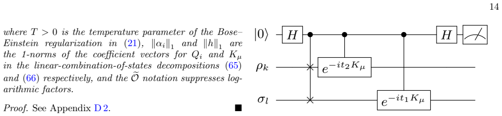
Proof of Proposition 8 In this section, we provide the full mathematical derivation proving that the classical aggregation of measurements from the quantum circuit in Figure 1 yields an unbiased estimate of the Bose–Einstein thermal traceTr[XT (µ)Qi]. The proof proceeds in three steps: (1) state evolution of the Hadamard test, (2) the Joint Monte Carlo ex...
-
[73]
Computational Complexity of Algorithm 2 In this section, we derive the computational complexity of estimating the thermal traceTr[XT (µ)Qi]using Algo- rithm 2. To guarantee a total additive error bounded byε, we partition the error budget equally among three sources of algorithmic approximation: the truncation of the infinite geometric series (ε/3), the t...
-
[74]
Thus, the algorithm evaluates the Bose–Einstein trace with a polynomial scaling in all physical parameters
By Hoeffding’s inequality, the number of independent shotsN(m) shots required to suppress the statistical variance of the mean to the target precisionO(ε/M)scales as: N(m) shots =O Var(Y) (ε/M)2 =O M2 ∥αi∥2 1 ε2 ! .(D23) 38 Step 5: Total Asymptotic Complexity.The total algorithmic runtime is the sum of the gate operations across all shots for allMterms in...
-
[75]
Proof of Correctness for the Hessian Estimation Algorithm In this section, we prove that the quantum circuit in Figure 2 yields an unbiased estimate of the Hessian matrix elementH ij. The proof proceeds in three steps: (1) state evolution of the controlled-SWAP circuit, (2) the Joint Monte Carlo expectation over time, continuous parameters, and state indi...
-
[76]
Because the algorithmic structure parallels the gradient estimator, we extend the error partitioning logic from Appendix D2 to the double geometric series
Computational Complexity of Algorithm 3 In this section, we derive the computational complexity of estimating the Hessian matrix elementHij using Algo- rithm 3. Because the algorithmic structure parallels the gradient estimator, we extend the error partitioning logic from Appendix D2 to the double geometric series. We allocate the total additive error bud...
-
[77]
41 Appendix E: Bose–Einstein relative entropy: proofs of properties
By Hoeffding’s inequality, the number of independent shots required to suppress the statistical variance of the mean to the target precisionO(ε/M2)scales as: N(m1,m2) shots =O Var(Y) (ε/M2)2 =O M4 ∥αi∥2 1 ∥αj∥2 1 ε2 ! .(D45) Step 5: Total Asymptotic Complexity.The total algorithmic runtime is the sum of the gate operations across all shots for allM2 terms...
-
[78]
Proof of Proposition 11 (Faithfulness and Support) Proof.We first prove the non-negativityD BE(X∥Y)≥0, with equality if and only ifX=Y. As established in Remark 5, the Bose–Einstein relative entropy coincides with the matrix Bregman divergence generated by the trace functionF(X) = Tr[f(X)] =−S BE(X), where the underlying scalar function isf(x):=xlnx−(x+ 1...
-
[79]
Proof of Proposition 12 (Unitary Invariance) Proof.LetUbe a unitary, i.e.,U †U=U U † =I. SubstitutingU XU † andU Y U † into the definition of the Bose– Einstein relative entropy in (85), yields: DBE(U XU †∥U Y U†) =−S BE(U XU †) + Tr[(U XU† +I) ln(U Y U † +I)−U XU † ln(U Y U†)].(E7) Because the Bose–Einstein entropy, defined in (19), is evaluated as the t...
-
[80]
Because {|ϕj⟩}forms a complete basis,P j |ϕj⟩ ⟨ϕj|=I
Proof of Proposition 13 (Spectral Expansion) Proof.Given the spectral decompositionsX= P i xi|ψi⟩ ⟨ψi|andY= P j yj|ϕj⟩ ⟨ϕj|, we first expand the single- argument entropy−S BE(X)in the definition of the Bose–Einstein relative entropyD BE(X∥Y)in (85). Because {|ϕj⟩}forms a complete basis,P j |ϕj⟩ ⟨ϕj|=I. We can therefore insert this resolution of the identi...
discussion (0)
Sign in with ORCID, Apple, or X to comment. Anyone can read and Pith papers without signing in.