Semi-Supervised Hypothesis Testing by Betting on Predictions
Pith reviewed 2026-06-29 13:51 UTC · model grok-4.3
The pith
An e-statistic from predictions on unlabeled data creates anytime-valid sequential hypothesis tests under label or concept shift.
A machine-rendered reading of the paper's core claim, the machinery that carries it, and where it could break.
Core claim
We introduce an e-statistic and use it to construct a sequential test. Under standard distributional assumptions -- label shift or concept shift -- we establish that the test is anytime valid. Furthermore, we show that for binary data, the e-statistic has non-trivial power. Crucially, our approach retains these properties even when the underlying predictions are inaccurate.
What carries the argument
An e-statistic constructed by betting on predictions of Y from X on unlabeled samples.
If this is right
- The sequential test controls type I error at any time under the stated assumptions.
- It has non-trivial power against alternatives for binary data.
- It outperforms baseline methods and prediction-powered inference in simulations and LLM evaluation tasks.
- These advantages remain with limited unlabeled data and low-accuracy predictions.
Where Pith is reading between the lines
- The betting construction could be adapted to test other functionals of the conditional distribution beyond the basic hypotheses considered.
- Similar use of predictions might increase power in other semi-supervised testing problems that currently rely only on labeled samples.
- Applying the method to datasets with independently verified label shift would provide a direct check on the reported power gains.
Load-bearing premise
The data distribution satisfies either label shift or concept shift.
What would settle it
A simulation or real-data case in which the sequential test exceeds its rejection threshold under the null hypothesis at a rate higher than the nominal alpha, while label shift or concept shift holds.
Figures


read the original abstract
We introduce a testing-by-betting framework that leverages predictions on unlabeled data to enhance the power of sequential hypothesis testing. Given limited samples from the joint distribution of $(X,Y)$, and additional unlabeled samples from the marginal of $X$, we ask how unlabeled data can be used to hypothesize about the distribution of $Y$, and the conditional distribution of $Y\mid X$. We introduce an e-statistic and use it to construct a sequential test. Under standard distributional assumptions -- label shift or concept shift -- we establish that the test is anytime valid. Furthermore, we show that for binary data, the e-statistic has non-trivial power. Crucially, our approach retains these properties even when the underlying predictions are inaccurate. Through simulations and applications to large language models evaluation, we demonstrate power gains over baseline approaches, including prediction-powered inference. These gains persist even with relatively limited unlabeled data and when predictions have low accuracy due to weak correlation between $X$ and $Y$.
Editorial analysis
A structured set of objections, weighed in public.
Referee Report
Summary. The paper introduces a testing-by-betting framework for semi-supervised sequential hypothesis testing. Given limited labeled samples from the joint (X,Y) distribution and additional unlabeled samples from the marginal of X, it constructs an e-statistic from predictions on the unlabeled X's. Under label shift or concept shift, the resulting e-process is shown to be a supermartingale (anytime valid). For binary Y the e-statistic is claimed to have non-trivial power even when the predictor is arbitrarily inaccurate. Simulations and an LLM-evaluation application demonstrate power gains over baselines including prediction-powered inference, with the gains persisting under limited unlabeled data and low-accuracy predictions.
Significance. If the validity and power claims hold, the work would extend the betting/e-process literature to a practically relevant semi-supervised regime while preserving the key robustness property that validity does not require predictor accuracy. The ability to obtain power improvements from unlabeled data even when X and Y are only weakly correlated is a potentially useful contribution for sequential testing in machine-learning evaluation and other label-scarce domains.
minor comments (3)
- The abstract and introduction state that the e-statistic is constructed from predictions on unlabeled X samples, but the precise functional form (how the prediction is turned into the betting payoff) is not visible in the provided abstract; a short explicit definition or reference to the relevant equation in §3 would improve readability.
- The power claim is stated for binary data; it would be helpful to clarify in the main text whether the non-trivial power result extends to the multi-class or continuous-Y settings mentioned in the broader framework, or whether it is deliberately restricted.
- The experimental section compares against prediction-powered inference; a brief discussion of why the betting construction yields gains even when the underlying predictor is weak would strengthen the narrative (currently only shown empirically).
Simulated Author's Rebuttal
We thank the referee for the positive assessment of our work, the recognition of its potential contributions to semi-supervised sequential testing, and the recommendation for minor revision. No specific major comments were provided in the report.
Circularity Check
No significant circularity detected
full rationale
The paper constructs an e-statistic from predictions on unlabeled X samples and proves the resulting e-process is a supermartingale (hence the sequential test is anytime valid) under the external distributional assumptions of label shift or concept shift. These assumptions are standard and independent of the paper's fitted quantities or prior self-citations. No equation reduces a claimed prediction to a fitted parameter by construction, no uniqueness theorem is imported from the authors' prior work, and the non-trivial power result for binary Y is stated to hold even for inaccurate predictors. The derivation chain is therefore self-contained against external benchmarks rather than circular.
Axiom & Free-Parameter Ledger
Reference graph
Works this paper leans on
-
[1]
PPI++: Efficient Prediction-Powered Inference
Angelopoulos, A. N., Bates, S., Fannjiang, C., Jordan, M. I., and Zrnic, T. Prediction-powered inference.Science, 382 (6671):669–674, 2023a. Angelopoulos, A. N., Duchi, J. C., and Zrnic, T. PPI++: Efficient prediction-powered inference.arXiv preprint arXiv:2311.01453, 2023b. Cobbe, K., Kosaraju, V ., Bavarian, M., Chen, M., Jun, H., Kaiser, L., Plappert, ...
work page internal anchor Pith review Pith/arXiv arXiv
-
[2]
Csillag, D., Struchiner, C. J., and Goedert, G. T. Prediction- powered e-values.arXiv preprint arXiv:2502.04294,
-
[3]
DeepSeek-R1: Incentivizing Reasoning Capability in LLMs via Reinforcement Learning
URL https://arxiv.org/abs/2501.12948. Ding, F., Hardt, M., Miller, J., and Schmidt, L. Retiring adult: New datasets for fair machine learning.Advances in neural information processing systems, 34:6478–6490,
work page internal anchor Pith review Pith/arXiv arXiv
-
[4]
Grattafiori, A., Dubey, A., Jauhri, A., Pandey, A., Kadian, A., Al-Dahle, A., Letman, A., Mathur, A., Schelten, A., Vaughan, A., et al. The llama 3 herd of models.arXiv preprint arXiv:2407.21783,
work page internal anchor Pith review Pith/arXiv arXiv
-
[5]
Tabpfn: A transformer that solves small tabular classifica- tion problems in a second
Hollmann, N., M¨uller, S., Eggensperger, K., and Hutter, F. Tabpfn: A transformer that solves small tabular classifica- tion problems in a second. InThe Eleventh International Conference on Learning Representations, ICLR 2023,
2023
-
[6]
Etude critique de la notion de collectif, gauthier- villars, paris, 1939.Monographies des Probabilit ´es
Ville, J. Etude critique de la notion de collectif, gauthier- villars, paris, 1939.Monographies des Probabilit ´es. Cal- cul des Probabilit´es et ses Applications,
1939
- [7]
-
[8]
Yang, A., Yang, B., Zhang, B., Hui, B., Zheng, B., Yu, B., Li, C., Liu, D., Huang, F., Wei, H., Lin, H., Yang, J., Tu, J., Zhang, J., Yang, J., Yang, J., Zhou, J., Lin, J., Dang, K., Lu, K., Bao, K., Yang, K., Yu, L., Li, M., Xue, M., Zhang, P., Zhu, Q., Men, R., Lin, R., Li, T., Xia, T., Ren, X., Ren, X., Fan, Y ., Su, Y ., Zhang, Y ., Wan, Y ., Liu, Y ....
work page internal anchor Pith review Pith/arXiv arXiv
-
[9]
Background A.1
10 Semi-Supervised Hypothesis Testing by Betting on Predictions A. Background A.1. First-order stochastic dominance (FOSD). The notion of stochastic order and FOSD in particular are at the core of this work. Formally, let X and Y be real-valued random variables with cumulative distribution functions FX(t) =P(X≤t) and FY (t) =P(Y≤t) . We say that Y first-o...
2007
-
[10]
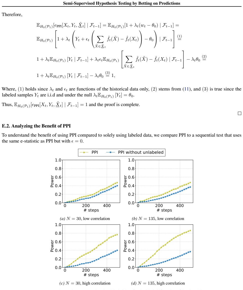
, given a sequence (X1, Y1, ˜X 1), . . . ,(Xt, Yt, ˜X t) of labeled and unlabeled data, we define the following betting procedure: At each step t, we betλ t of our wealth against the null and receive the payoff: ePPI[Xt, Yt, ˜X t] = 1 +λ t(wt −θ null Y ),(9) whereλ t ∈[−1/2,1/2]andw t is the PPI estimator for the mean ofY: wt =Y t +ϵ t 1 N X X∈ ˜X t ˆ...
2023
-
[11]
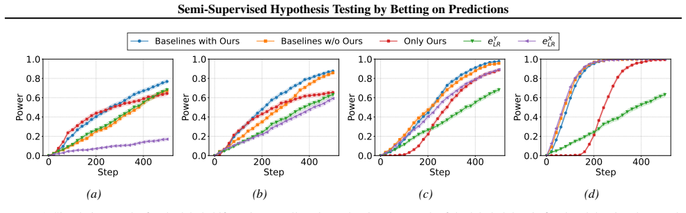
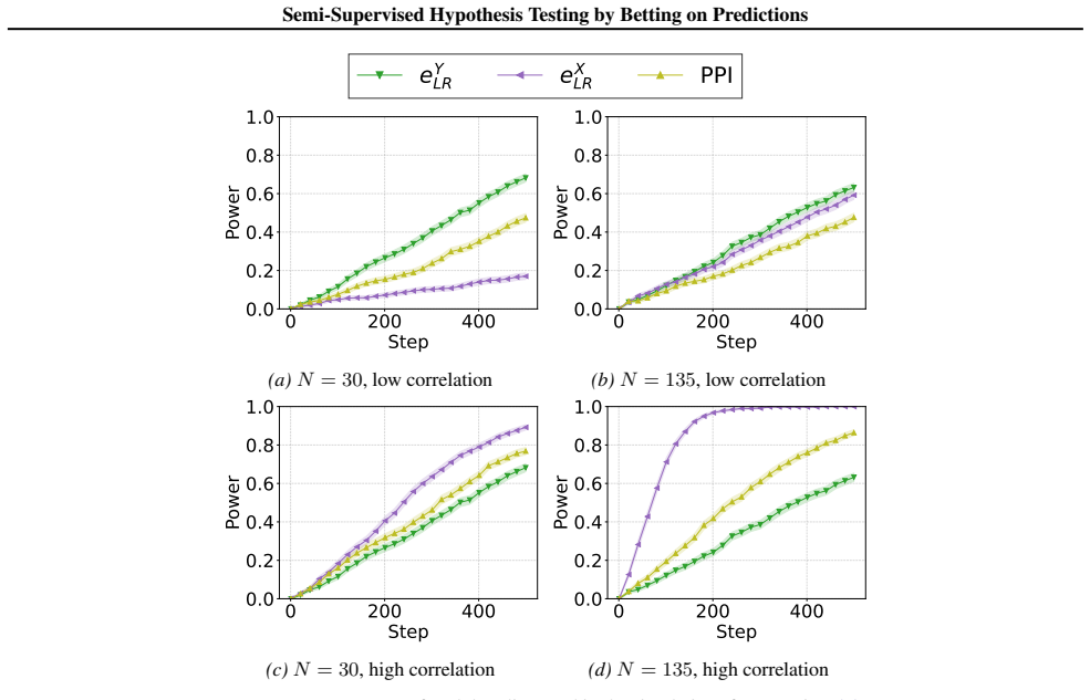
= 0.9. 27 Semi-Supervised Hypothesis Testing by Betting on Predictions eY LR eX LR PPI 0 200 400 Step 0.0 0.2 0.4 0.6 0.8 1.0Power (a)N= 30, low correlation 0 200 400 Step 0.0 0.2 0.4 0.6 0.8 1.0Power (b)N= 135, low correlation 0 200 400 Step 0.0 0.2 0.4 0.6 0.8 1.0Power (c)N= 30, high correlation 0 200 400 Step 0.0 0.2 0.4 0.6 0.8 1.0Power (d)N= 135, hig...
2021
discussion (0)
Sign in with ORCID, Apple, or X to comment. Anyone can read and Pith papers without signing in.