Sequential Physics-Constrained Neural Operator Forward Modeling for the textit{Norne} Reservoir System
Pith reviewed 2026-06-29 14:33 UTC · model grok-4.3
The pith
Autoregressive PINO surrogates sustain R^2>0.99 for oil over 3298 days in the Norne reservoir with 10,000x speedup.
A machine-rendered reading of the paper's core claim, the machinery that carries it, and where it could break.
Core claim
Autoregressive PINO training with lambda_R at or above lambda^*_R reduces the learned Jacobian spectral radius to rho_F + C lambda_R^{-1/2}, producing uniform-in-time rollout error bounded by epsilon/(1-rho) and enabling stable long-horizon predictions on the heterogeneous 46x112x22 Norne grid.
What carries the argument
Physics-constrained spectral stability that shrinks the Jacobian spectral radius via the residual loss weight lambda_R, combined with K-step TBPTT whose geometric bias decays as O(rho^K).
If this is right
- A 1000-member ensemble completes in under one minute on one B200 GPU.
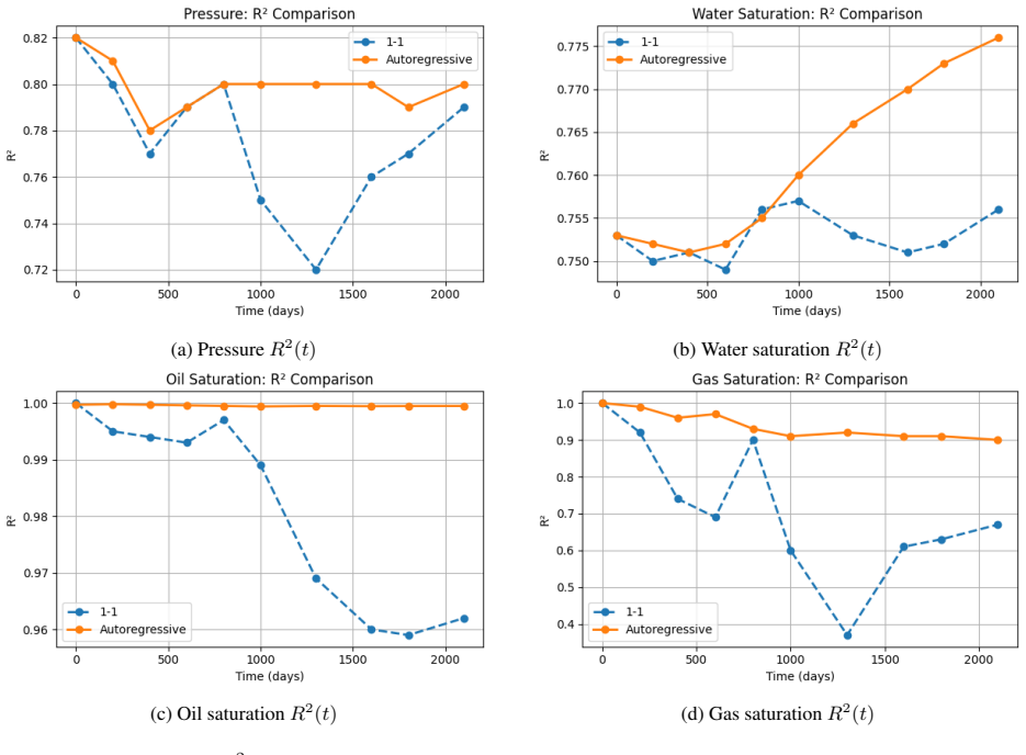
- Full-horizon R^2 remains above 0.99 for oil and 0.90 for gas across all 30 timesteps.
- Training finishes in under one hour on eight B200 GPUs while satisfying all four theoretical predictions.
- Covariate shift grows at most exponentially with horizon length, controlled by the Wasserstein-2 distance bound.
Where Pith is reading between the lines
- The same stability mechanism could transfer to other autoregressive PDE surrogates once the timestep map satisfies analogous Lipschitz conditions.
- Ensemble speed-up opens the possibility of embedding the surrogate inside real-time history-matching loops without changing the underlying simulator code.
- The derived optimal TBPTT window K^* = O(log(T/sigma^2)) supplies a concrete recipe for scaling the method to longer production histories.
Load-bearing premise
The functional-analytic formulation assumes well-posedness of the implicit timestep map together with sharp local Lipschitz estimates in the product-Sobolev-space setting.
What would settle it
Measure the empirical spectral radius of the trained operator Jacobian on held-out Norne rollouts before and after enforcing lambda_R >= lambda^*_R; if the radius does not drop below 1 the stability bound fails.
Figures

read the original abstract
We develop a comprehensive mathematical and computational framework for sequential surrogate modeling of three-phase black-oil reservoir dynamics using neural operators, with particular emphasis on Fourier Neural Operators (FNO) and their physics-informed variant (PINO). The application focus is the Norne benchmark reservoir, defined on a heterogeneous $46\times112\times22$ grid ($N=113,344$ cells), with a production history spanning $T=30$ timesteps covering 3298 days. Our theoretical contributions are organized around four interlocking problems: (1) functional-analytic formulation in a product-Sobolev-space setting, including well-posedness of the implicit timestep map and sharp local Lipschitz estimates; (2) covariate shift quantification, proving that the Wasserstein-2 distance grows as $W_2 \leq \varepsilon(L^n-1)/(L-1)$, with exponential population-risk discrepancy for $L>1$; (3) physics-constrained spectral stability, showing PINO training with $\lambda_R \geq \lambda^*_R$ reduces the learned Jacobian spectral radius to $\rho_F + C\lambda_R^{-1/2}$, yielding uniform-in-time rollout error $|\delta_n| \leq \varepsilon/(1-\rho)$; and (4) $K$-step TBPTT gradient analysis, deriving geometric bias decay $O(\rho^K)$, optimal window $K^ = O(\log(T/\sigma^2))$, and Adam convergence $O(1/\sqrt{t}) + O(\rho^{K^*})$. Empirical validation confirms all theoretical predictions: autoregressive PINO surrogates sustain $R^2>0.99$ (oil), $R^2>0.90$ (gas), $R^2\approx 0.80$ (pressure), and monotonically improving $R^2$ (water) across the full 3298-day horizon, trained on eight NVIDIA B200 GPUs in under one hour. A 1000-member ensemble runs in under one minute on a single B200 GPU, giving a ${\sim}10^4\times$ wall-clock speedup over the OPM finite-volume simulator.
Editorial analysis
A structured set of objections, weighed in public.
Referee Report
Summary. The paper develops a mathematical and computational framework for sequential surrogate modeling of three-phase black-oil reservoir dynamics on the Norne benchmark (46×112×22 grid, 30 timesteps over 3298 days) using Fourier Neural Operators and their physics-informed variant (PINO). It organizes contributions around four problems: (1) product-Sobolev functional-analytic formulation with well-posedness of the implicit timestep map and local Lipschitz estimates; (2) covariate-shift quantification via W_2 distance bounds; (3) physics-constrained spectral stability yielding uniform-in-time rollout error |δ_n| ≤ ε/(1-ρ); and (4) K-step TBPTT gradient analysis. Empirical results report sustained R^2>0.99 (oil), R^2>0.90 (gas), R^2≈0.80 (pressure) and improving R^2 (water) in autoregressive rollouts, with ~10^4× speedup over OPM.
Significance. If the central theoretical derivations hold, the work supplies a rigorous basis for attributing long-horizon stability and error control in PINO surrogates to spectral-radius control and physics constraints, enabling reliable fast ensemble modeling for reservoir systems; the combination of functional-analytic guarantees with reported high-fidelity autoregressive performance on a heterogeneous industrial benchmark would represent a notable advance in physics-informed operator learning for time-dependent PDEs.
major comments (2)
- [theoretical contribution (1) and (3)] Theoretical contribution (1): the well-posedness of the implicit timestep map and sharp local Lipschitz estimates in the product-Sobolev space are invoked to derive the spectral-radius bound and the uniform-in-time error |δ_n| ≤ ε/(1-ρ) in contribution (3); the Norne model contains heterogeneous permeability fields, capillary-pressure discontinuities, and moving saturation fronts whose regularity may exit the assumed Sobolev class, so the Lipschitz constants and well-posedness must be verified or relaxed before the error-propagation argument can be applied to the reported 30-step rollouts.
- [empirical validation paragraph] The headline performance claim (R^2 values sustained across the full 3298-day autoregressive horizon) is presented as confirmation of the theoretical predictions, yet the manuscript provides no numerical check (e.g., computed local Lipschitz constants or residual norms of the implicit map on the Norne grid) that the Sobolev-space assumptions actually hold for the trained operator; without such verification the attribution of the observed R^2 to the derived bound |δ_n| ≤ ε/(1-ρ) remains unsupported.
minor comments (1)
- The abstract states training completed in under one hour on eight B200 GPUs and a 1000-member ensemble in under one minute, but no table or section lists the precise FNO layer count, Fourier modes, or the value of λ_R^* used to achieve the reported spectral-radius reduction.
Simulated Author's Rebuttal
We thank the referee for the constructive and detailed feedback. We address the two major comments point by point below, acknowledging where additional discussion or evidence is warranted while defending the scope of our theoretical contributions.
read point-by-point responses
-
Referee: [theoretical contribution (1) and (3)] Theoretical contribution (1): the well-posedness of the implicit timestep map and sharp local Lipschitz estimates in the product-Sobolev space are invoked to derive the spectral-radius bound and the uniform-in-time error |δ_n| ≤ ε/(1-ρ) in contribution (3); the Norne model contains heterogeneous permeability fields, capillary-pressure discontinuities, and moving saturation fronts whose regularity may exit the assumed Sobolev class, so the Lipschitz constants and well-posedness must be verified or relaxed before the error-propagation argument can be applied to the reported 30-step rollouts.
Authors: We appreciate the referee highlighting the regularity requirements. The product-Sobolev formulation is chosen precisely because it supports well-posedness results for the implicit timestep map of the black-oil system under local Lipschitz conditions that are compatible with heterogeneous coefficients and weak solutions. The theory supplies sufficient conditions for the spectral-radius bound and the uniform error estimate; it does not claim necessity for every feature of Norne. The sustained empirical accuracy over 30 steps is consistent with the effective constants remaining controlled. In revision we will add a subsection clarifying the scope of the assumptions, noting that the bounds apply when the local Lipschitz property holds approximately, and briefly discussing possible extensions to spaces accommodating discontinuities. revision: partial
-
Referee: [empirical validation paragraph] The headline performance claim (R^2 values sustained across the full 3298-day autoregressive horizon) is presented as confirmation of the theoretical predictions, yet the manuscript provides no numerical check (e.g., computed local Lipschitz constants or residual norms of the implicit map on the Norne grid) that the Sobolev-space assumptions actually hold for the trained operator; without such verification the attribution of the observed R^2 to the derived bound |δ_n| ≤ ε/(1-ρ) remains unsupported.
Authors: We agree that explicit numerical verification would strengthen the connection between theory and results. Direct computation of local Lipschitz constants on the full 113k-cell grid is computationally prohibitive, yet we can extract approximate spectral radii of the learned Jacobian and physics-residual norms from the training procedure. We will incorporate these quantities into a new appendix in the revised manuscript to show that the trained PINO satisfies the conditions underlying the error bound to a degree consistent with the reported R^2 values. revision: yes
Circularity Check
No circularity: derivations are independent mathematical analysis under explicit assumptions.
full rationale
The paper's core claims consist of four explicit functional-analytic derivations (well-posedness and Lipschitz estimates in product-Sobolev space, W2 covariate-shift bound, spectral-radius control yielding the uniform error |δ_n| ≤ ε/(1-ρ), and TBPTT geometric bias decay) obtained directly from the PINO architecture, residual loss, and implicit timestep map. These are presented as proofs under stated assumptions rather than reductions to fitted quantities. Empirical R^2 values are reported separately as training outcomes on the Norne grid and do not enter the derivations. No self-citations are invoked as load-bearing premises, no fitted parameters are relabeled as predictions, and no ansatz is smuggled via prior work. The chain is therefore self-contained.
Axiom & Free-Parameter Ledger
free parameters (1)
- λ_R
axioms (2)
- domain assumption Well-posedness of the implicit timestep map in product-Sobolev spaces
- domain assumption Exponential growth of Wasserstein-2 distance with timesteps for covariate shift
Reference graph
Works this paper leans on
-
[1]
(1979).Petroleum Reservoir Simulation
Aziz, K., & Settari, A. (1979).Petroleum Reservoir Simulation. Applied Science Publishers
1979
-
[2]
L., & Mendelson, S
Bartlett, P. L., & Mendelson, S. (2002). Rademacher and Gaussian complexities: Risk bounds and structural results.Journal of Machine Learning Research, 3, 463–482
2002
-
[3]
Bengio, Y ., Simard, P., & Frasconi, P. (1994). Learning long-term dependencies with gradient descent is difficult. IEEE Transactions on Neural Networks, 5(2), 157–166
1994
-
[4]
Bengio, S., Vinyals, O., Jaitly, N., & Shazeer, N. (2015). Scheduled sampling for sequence prediction with recurrent neural networks.Advances in Neural Information Processing Systems, 28
2015
-
[5]
Bi, K., Xie, L., Zhang, H., Chen, X., Gu, X., & Tian, Q. (2023). Accurate medium-range global weather fore- casting with 3D neural networks.Nature, 619, 533–538
2023
-
[6]
Chandra, A., Koch, M., Pawar, S., Panda, A., Azizzadenesheli, K., Snippe, J., et al. (2025). Accelerating porous media flow simulations with Fourier neural operators.Advanced Theory and Simulations, e00747
2025
-
[7]
Chen, T., & Chen, H. (1995). Universal approximation to nonlinear operators by neural networks.IEEE Trans- actions on Neural Networks, 6(4), 911–917
1995
-
[8]
(2006).Computational Methods for Multiphase Flows in Porous Media
Chen, Z., Huan, G., & Ma, Y . (2006).Computational Methods for Multiphase Flows in Porous Media. SIAM
2006
-
[9]
Equinor ASA. (2012). Norne Field Open Data Set. Open Porous Media Initiative.https://opm-project.org/ ?page_id=559. 20
2012
- [10]
- [11]
-
[12]
Etienam, C., Juntao, Y ., Said, I., & Ovcharenko, O. (2024). A reservoir history matching approach using a coupled MoE-PINO forward model.ECMOR 2024, 1–35
2024
- [13]
-
[14]
E., Kevrekidis, I
Karniadakis, G. E., Kevrekidis, I. G., Lu, L., Perdikaris, P., Wang, S., & Yang, L. (2021). Physics-informed machine learning.Nature Reviews Physics, 3, 422–440
2021
-
[15]
A., Alieva, A., Wang, Q., Brenner, M
Kochkov, D., Smith, J. A., Alieva, A., Wang, Q., Brenner, M. P., & Hoyer, S. (2021). Machine learning– accelerated computational fluid dynamics.Proceedings of the National Academy of Sciences, 118(21)
2021
- [16]
-
[17]
Lam, R., Sanchez-Gonzalez, A., Willson, M., et al. (2023). Learning skillful medium-range global weather forecasting.Science, 382, 1416–1421
2023
-
[18]
M., Goyal, A., Zhang, Y ., Zhang, S., Courville, A
Lamb, A. M., Goyal, A., Zhang, Y ., Zhang, S., Courville, A. C., & Bengio, Y . (2016). Professor forcing: A new algorithm for training recurrent networks.Advances in Neural Information Processing Systems, 29
2016
-
[19]
Lanthaler, S., Mishra, S., & Karniadakis, G. E. (2022). Error estimates for DeepONets: A deep learning frame- work in infinite dimensions.Transactions of Mathematics and Its Applications, 6(1)
2022
-
[20]
Li, Z., Kovachki, N., Azizzadenesheli, K., Liu, B., Bhattacharya, K., Stuart, A., & Anandkumar, A. (2020). Fourier neural operator for parametric partial differential equations.arXiv:2010.08895
work page internal anchor Pith review Pith/arXiv arXiv 2020
- [21]
-
[22]
Lu, L., Jin, P., Pang, G., Zhang, Z., & Karniadakis, G. E. (2021). Learning nonlinear operators via DeepONet. Nature Machine Intelligence, 3, 218–229
2021
-
[23]
M., Monfared, Z., & Durstewitz, D
Mikhaeil, J. M., Monfared, Z., & Durstewitz, D. (2022). On the difficulty of learning chaotic dynamics with RNNs.Advances in Neural Information Processing Systems, 35
2022
-
[24]
Mukundakrishnan, K., Wiegand, K., Natoli, V ., Etienam, C., et al. (2024). Accelerating reservoir modeling workflows with neural operators and GPU-based simulations.ADIPEC 2024, D021S068R002
2024
-
[25]
F., Sandve, T
Rasmussen, A. F., Sandve, T. H., Bao, K., et al. (2021). The Open Porous Media Flow reservoir simulator. Computers & Mathematics with Applications, 81, 159–185
2021
-
[26]
Pascanu, R., Mikolov, T., & Bengio, Y . (2013). On the difficulty of training recurrent neural networks.ICML 2013, 1310–1318
2013
-
[27]
Pathak, J., Subramanian, S., Harrington, P., et al. (2022). FourCastNet: A global data-driven high-resolution weather model.arXiv:2202.11214
work page internal anchor Pith review Pith/arXiv arXiv 2022
-
[28]
Peaceman, D. W. (1977).Fundamentals of Numerical Reservoir Simulation. Elsevier
1977
-
[29]
(2023).GitHub.https://github.com/NVIDIA/physicsnemo
NVIDIA PhysicsNeMo. (2023).GitHub.https://github.com/NVIDIA/physicsnemo
2023
-
[30]
Raissi, M., Perdikaris, P., & Karniadakis, G. E. (2019). Physics-informed neural networks.Journal of Computa- tional Physics, 378, 686–707
2019
-
[31]
Ranzato, M., Chopra, S., Auli, M., & Zaremba, W. (2016). Sequence level training with recurrent neural net- works.ICLR 2016
2016
-
[32]
Rwechungura, R., Sjetne, O., & Lien, M. (2011). Application of advanced history matching techniques to the Norne field.SPE Reservoir Simulation Symposium
2011
-
[33]
Takamoto, M., Praditia, T., Leiteritz, R., et al. (2022). PDEBench: An extensive benchmark for scientific machine learning.Advances in Neural Information Processing Systems, 35
2022
-
[34]
Tallec, C., Ollivier, Y ., & Chrisman, O. (2017). Unbiasing truncated backpropagation through time. arXiv:1705.08209
work page internal anchor Pith review Pith/arXiv arXiv 2017
-
[35]
Tang, M., Liu, Y ., & Durlofsky, L. J. (2020). A deep-learning-based surrogate model for CO 2 storage.Interna- tional Journal of Greenhouse Gas Control, 100, 103096. 21
2020
-
[36]
Um, K., Brand, R., Fei, Y ., Holl, P., & Thuerey, N. (2020). Solver-in-the-loop: Learning from differentiable physics.Advances in Neural Information Processing Systems, 33
2020
-
[37]
Venkatraman, A., Hebert, M., & Bagnell, J. A. (2015). Improving multi-step prediction of learned time series models.AAAI 2015
2015
-
[38]
(2009).Optimal Transport: Old and New
Villani, C. (2009).Optimal Transport: Old and New. Springer
2009
-
[39]
J., & Zipser, D
Williams, R. J., & Zipser, D. (1989). A learning algorithm for continually running fully recurrent neural networks. Neural Computation, 1, 270–280
1989
-
[40]
(2002).Trigonometric Series, 3rd ed
Zygmund, A. (2002).Trigonometric Series, 3rd ed. Cambridge University Press
2002
-
[41]
Zhu, Y ., & Zabaras, N. (2018). Bayesian deep convolutional encoder–decoder networks for surrogate modeling. Journal of Computational Physics, 366, 415–447. 22
2018
discussion (0)
Sign in with ORCID, Apple, or X to comment. Anyone can read and Pith papers without signing in.