Analytic Bootstrap for O(N) Boundary Conformal Field Theories with Interacting Boundaries
Pith reviewed 2026-06-29 10:45 UTC · model grok-4.3
The pith
Universal constraints from analytic bootstrap express infinitely many operator expansions in O(N) boundary CFTs using only a finite set of inputs.
A machine-rendered reading of the paper's core claim, the machinery that carries it, and where it could break.
Core claim
By deriving universal constraints on conformal data, the analytic bootstrap shows that infinitely many operator expansions can be expressed in terms of a finite set of inputs. Complementing this with perturbative renormalization-group analysis identifies totally new boundary fixed points in d=4-ε, including non-unitary ones generated by a boundary cubic coupling, with their conformal data computed to leading order. The solution in d=3-ε extracts the boundary conformal data for the tricritical O(N) model for the first time.
What carries the argument
Universal constraints on conformal data derived from the analytic bootstrap, which reduce infinitely many boundary operator expansions to a finite set of inputs.
If this is right
- New boundary fixed points exist in d=4-ε generated by boundary cubic coupling, including non-unitary ones.
- Conformal data for these fixed points is computed to leading order in epsilon.
- Boundary conformal data for the tricritical O(N) model is obtained in d=3-ε.
- Infinitely many operator expansions are determined by finite inputs via the constraints.
Where Pith is reading between the lines
- The approach may extend to other interacting boundary theories beyond O(N) symmetry.
- Non-unitary fixed points could connect to studies of non-unitary conformal field theories in lower dimensions.
- Future work might test these predictions against lattice simulations of boundary models.
Load-bearing premise
The analytic bootstrap and epsilon-expansion remain valid when applied to O(N) theories with an added boundary cubic coupling without extra constraints or inconsistencies arising from the boundary interactions.
What would settle it
A lattice simulation or numerical study of the tricritical O(N) model in three dimensions that measures boundary scaling dimensions or OPE coefficients differing from the epsilon-expansion predictions would falsify the extracted conformal data.
Figures

read the original abstract
We investigate $O(N)$ boundary conformal field theories (BCFTs) with boundary interactions in $d=4-\epsilon$ and $d=3-\epsilon$ employing the analytic bootstrap. By deriving universal constraints on conformal data, we show that infinitely many operator expansions can be expressed in terms of a finite set of inputs. Complementing the analytic bootstrap with a perturbative renormalization-group analysis, we identify totally new boundary fixed points in $d=4-\epsilon$, including non-unitary ones, generated by a boundary cubic coupling, and compute their conformal data to leading order. Moreover, we leverage our solution in $d=3-\epsilon$ to extract, for the first time, the boundary conformal data for the tricritical $O(N)$ model. Altogether, our approach provides a unified prescription for BCFTs with interacting boundaries and streamlines the determination of bulk and boundary operator expansions.
Editorial analysis
A structured set of objections, weighed in public.
Referee Report
Summary. The manuscript investigates O(N) boundary conformal field theories with boundary interactions using the analytic bootstrap in d=4-ε and d=3-ε. It derives universal constraints on conformal data showing that infinitely many operator expansions reduce to a finite set of inputs, complements this with perturbative RG analysis to identify new boundary fixed points (including non-unitary ones) generated by a boundary cubic coupling and compute their data to leading order, and extracts boundary conformal data for the tricritical O(N) model in d=3-ε, providing a unified prescription for such BCFTs.
Significance. If the derivations hold, this supplies a streamlined method for determining bulk and boundary operator expansions in interacting BCFTs, with the first extraction of tricritical boundary data and identification of new fixed points representing concrete advances. The combination of analytic bootstrap constraints with RG matching is a methodological strength that could extend to other boundary deformations.
major comments (2)
- [Abstract and §3 (assumed bootstrap setup)] The central claim that the analytic bootstrap yields universal constraints reducing infinitely many OPEs to finite inputs (as stated in the abstract) requires explicit verification that the crossing equations close consistently under the added boundary cubic deformation; without a dedicated section deriving the modified crossing kernel or showing the reduction explicitly, it is unclear if this holds beyond the free-boundary case.
- [§4 (RG analysis and fixed-point identification)] For the new fixed points in d=4-ε, the leading-order conformal data computation via combined bootstrap and RG must specify how the boundary cubic coupling affects the beta functions and anomalous dimensions; if the non-unitary points rely on an unperturbed spectrum assumption, this needs explicit justification as it is load-bearing for the claim of 'totally new' fixed points.
minor comments (2)
- Notation for boundary operators and their dimensions should be standardized across sections to avoid ambiguity between bulk and boundary quantities.
- [Abstract] The abstract would benefit from a brief mention of the key technical inputs (e.g., the form of the crossing equations or the epsilon-expansion order) to improve readability.
Simulated Author's Rebuttal
We thank the referee for their positive assessment of the work and for the detailed, constructive comments. We respond to each major comment below, indicating where revisions will be made for clarity.
read point-by-point responses
-
Referee: [Abstract and §3 (assumed bootstrap setup)] The central claim that the analytic bootstrap yields universal constraints reducing infinitely many OPEs to finite inputs (as stated in the abstract) requires explicit verification that the crossing equations close consistently under the added boundary cubic deformation; without a dedicated section deriving the modified crossing kernel or showing the reduction explicitly, it is unclear if this holds beyond the free-boundary case.
Authors: In §3 we derive the universal constraints for the interacting-boundary case by solving the crossing equations after including the boundary operators generated by the cubic deformation. The reduction to a finite set of inputs follows from the structure of the modified crossing kernel, whose contributions from higher operators are fixed by the RG matching conditions at the fixed point. To make this explicit, we will add a dedicated subsection that derives the modified crossing kernel step by step and verifies the consistent closure of the equations. revision: yes
-
Referee: [§4 (RG analysis and fixed-point identification)] For the new fixed points in d=4-ε, the leading-order conformal data computation via combined bootstrap and RG must specify how the boundary cubic coupling affects the beta functions and anomalous dimensions; if the non-unitary points rely on an unperturbed spectrum assumption, this needs explicit justification as it is load-bearing for the claim of 'totally new' fixed points.
Authors: Section 4 computes the beta functions with the boundary cubic coupling included at leading order in ε and matches the resulting anomalous dimensions to the bootstrap data. The non-unitary fixed points are located by solving the full set of beta functions; their spectra receive perturbative corrections from the cubic term rather than assuming an unperturbed spectrum. We will expand the text to show the explicit dependence of the beta functions on the cubic coupling and to state the justification for the non-unitary cases. revision: yes
Circularity Check
No significant circularity
full rationale
The paper's central results follow from deriving crossing equations for O(N) BCFTs with boundary cubic interactions via the analytic bootstrap, then matching to perturbative RG flows in d=4-ε and d=3-ε. These steps rely on standard conformal block expansions and epsilon-expansion techniques applied to the deformed boundary action, without any load-bearing reduction to self-citations, fitted parameters renamed as predictions, or ansatze imported from prior author work. The new fixed points and conformal data are computed directly from the resulting equations, rendering the derivation self-contained against external CFT consistency conditions.
Axiom & Free-Parameter Ledger
Reference graph
Works this paper leans on
-
[1]
We have used the discontinuity of the hypergeometric function, Eq
P ( d 2 −1,0) n−1 − ξ+ 2 ξ , whereP (α,β) n denotes the Jacobi polynomial. We have used the discontinuity of the hypergeometric function, Eq. (A7), given in Appendix A 2. Therefore, using the orthogonality relation of Jacobi polynomials [67], Z 1 −1 dy(1−y) α(1 +y) βP (α,β) m (y)P (α,β) n (y) =δm,n 2α+β+1Γ(n+α+ 1)Γ(n+β+ 1) (2n+α+β+ 1)Γ(n+α+β+ 1)Γ(n+ 1) , ...
-
[2]
(49), we can first consider the expansion for ξ 1+ξ a , which serves as the building block
(52) For the first term in Eq. (49), we can first consider the expansion for ξ 1+ξ a , which serves as the building block. On the one hand, ξ 1+ξ a =ξ aP∞ l=0 (a)l l! (−1)lξl. On the other hand, the expansion in terms of the bulk conformal block reads ξ 1+ξ a =P∞ n=0 c′ a,nfb(2a+ 2n, ξ). We can further expand the bulk conformal blocks as power series ofξ,...
-
[3]
(53) Now, with these two results, Eqs. (52) and (53), it is straightforward to obtain the OPE coefficients for ⟨O(k)O(k)⟩ ˜λ2l∆ϕ+2n = Γ(k+ 1) Γ(l+ 1)Γ(k−l+ 1) slc′ l∆ϕ,n +δl,kαk,N ck∆ϕ,n,(54) withl= 0,1,· · ·, kandn= 0,1,· · ·. The expansion re- vealskdistinct families of conformal blocks correspond- ing to the scaling dimension ∆ = 2l∆ ϕ + 2n, where l= 1...
-
[4]
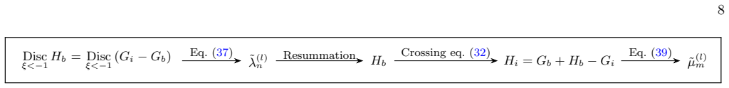
To avoid any ambiguity, we resum the conformal blocks inH i(ξ) using the BOE coefficients in Eq
, (68) where B′ 3 =− ˆ∆(1) 0 + 2∆(1) ϕ − 1 2∆(1) 0 , B ′ 4 = ∆(1) ϕ .(69) 12 In general, we expect the operations of taking discon- tinuities, performing series expansions, and resumming to commute. To avoid any ambiguity, we resum the conformal blocks inH i(ξ) using the BOE coefficients in Eq. (68) and check whether the result reproducesH i(ξ) in Eq. (65...
-
[5]
In the bulk, theN-component field, denoted asϕ i,i= 1, ..., N, trans- forms in the usual way under theO(N) group
RG calculation for theO(N)theory with cubic boundary interactions We consider anO(N) theory in ad-dimensional semi- infinite spaceR d + with a boundary atz= 0. In the bulk, theN-component field, denoted asϕ i,i= 1, ..., N, trans- forms in the usual way under theO(N) group. On the boundary, we consider anS N+1 invariant cubic interac- tion, whereϕ i fulfil...
-
[6]
Now, combining Eqs
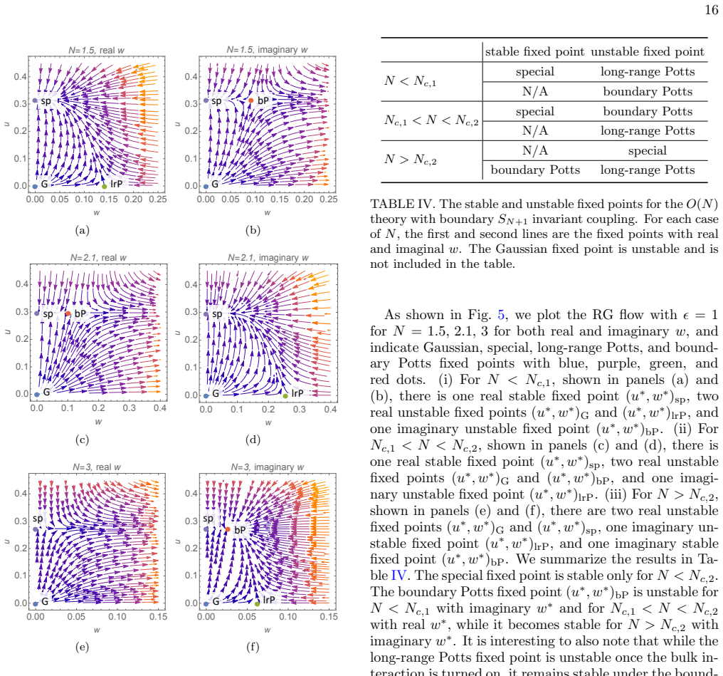
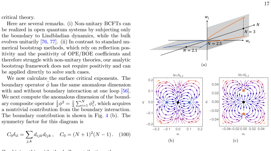
[75]. Now, combining Eqs. (91) (truncated atO(u 2)) and (98), we analyze the RG flow as a function ofN. Set- tingβ(u) =β(w) = 0 yields four distinct fixed points. Since for any fixed point (u ∗, w∗), the pair (u ∗,−w ∗) is equivalent, we restrict tow >0. The fixed points are (u∗, w∗)G = (0,0),(99) (u∗, w∗)sp = 3ϵ N+ 8 ,0 , (u∗, w∗)lrP = 0, 1 4 r ϵ (N+ 1) ...
-
[7]
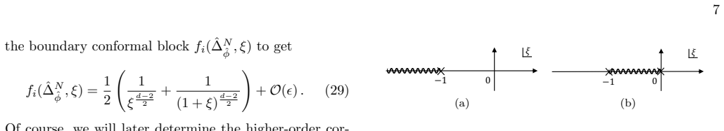
(98) vanishes
In particular, forN= 2 the coefficientC 5 in Eq. (98) vanishes. Consequently, any nontrivial fixed pointw ∗, if present, can only be resolved at the next order, i.e., at two loops. In the following, we plot the RG flow for both real and imaginarywat representative values ofN. stable fixed point unstable fixed point N < N c,1 special long-range Potts N/A b...
-
[8]
We compute the Green’s function to the first order
BOE coefficients at the long-range Potts/Yang-Lee fixed point We evaluate the OPE coefficient ˜λ(1) 0 at the long-range Potts/Yang-Lee fixed point. We compute the Green’s function to the first order. The boundary contribution is similar to the diagram (5) in Fig. 4 (a) with one of the external line removed, and gives I ′ = e−p(z1+z2) p − 1 4π2 . (103) The...
-
[9]
For the long-range Potts fixed point, λ0 =λ (0) 0 whilea (1) 0 ̸= 0, which gives ˜λ(1) 0 =λ (0) 0 a(1) 0,i ≡α ′
BOE coefficients at the boundary Potts/Yang-Lee fixed point For the BOE coefficient in the boundary Potts fixed point, ˜λ0, we first note that ˜λ0 =λ 0a0 =λ (0) 0 a(0) 0 + (λ(1) 0 a(0) 0 +λ (0) 0 a(1) 0 )ϵ+O(ϵ 2), (106) which indicates ˜λ(1) 0 =λ (1) 0 a(0) 0 +λ (0) 0 a(1) 0 .λ 0 is the bulk conformal data, that will not be affected by the bound- ary inte...
-
[10]
As discussed in Ref
Expansion of conformal blocks In this section, we calculate the series expansion of the hypergeometric function 2F1(a, b, c, x) toO(ϵ 2), with a=a 0+a1ϵ+a 2ϵ2, b=b 0+b1ϵ+b 2ϵ2, c=c 0+c1ϵ+c 2ϵ2. As discussed in Ref. [34], we use the integral represen- tation of hypergeometric functions: 2F1(a, b, c, z) = Γ(c) Γ(b)Γ(c−b) Z 1 0 dt tb−1(1−t) c−b−1 (1−tz) a . ...
-
[11]
Branch cut of special functions Here, we present the discontinuity of 2F1(a, b, c, x) withx >1 [105] lim ϵ→0+ 2F1(a, b, c, x+ iϵ) =e 2πi(a+b−c) 2F1 (a, b, c, x) + 2πieiπ(a+b−c)Γ(c) Γ(c−a)Γ(c−b)Γ(a+b−c+ 1) 2F1 (a, b, a+b−c+ 1,1−x), lim ϵ→0+ 2F1(a, b, c, x−iϵ) = 2F1(a, b, c, x),(A7)
-
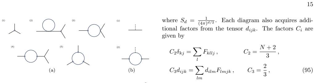
[12]
Appendix B: Normalization factor for the composite field We determine the normalization factorsf k,N in Eq
Discontinuity on the branch cut In this section, we list the discontinuities of some functions that are used in the main text to calculate Disc ξ<−1 (Gi(ξ)−G b(ξ)): Disc ξ<−1 logξ= Disc ξ<−1 log (1 +ξ) = 2πi,(A8) Disc ξ<−1 (logξ) 2 = 4πi log (−ξ), Disc ξ<−1 Li2(ξ) =−2πi log (−ξ), Disc ξ<−1 logξlog (1 +ξ) = 2πi(log (−ξ) + log (−1−ξ)). Appendix B: Normaliza...
-
[13]
Di Francesco, P
P. Di Francesco, P. Mathieu, and D. Senechal,Con- formal Field Theory, Graduate Texts in Contemporary Physics (Springer-Verlag, New York, 1997)
1997
-
[14]
D. J. Amit and V. Martin-Mayor,Field theory, the renormalization group, and critical phenomena: graphs to computers(World Scientific Publishing Company, 2005)
2005
-
[15]
J. L. Cardy, Nucl. Phys. B240, 514 (1984)
1984
-
[16]
Diehl, Phase transitions and and Critical Phenom- ena, edited by C
H. Diehl, Phase transitions and and Critical Phenom- ena, edited by C. Domb and JL Lebowitz10, 75 (1986)
1986
-
[17]
Affleck and A
I. Affleck and A. W. W. Ludwig, Phys. Rev. Lett.67, 161 (1991)
1991
-
[18]
R. Z. Bariev and L. Turban, Phys. Rev. B45, 10761 (1992)
1992
-
[19]
H. W. Diehl, Int. J. Mod. Phys. B11, 3503 (1997), arXiv:cond-mat/9610143
work page internal anchor Pith review Pith/arXiv arXiv 1997
-
[20]
Boundary Conformal Field Theory
J. Cardy, Boundary conformal field theory (2004), arXiv:hep-th/0411189 [hep-th]
work page internal anchor Pith review Pith/arXiv arXiv 2004
-
[21]
C. P. Herzog, K.-W. Huang, and K. Jensen, JHEP01, 162, arXiv:1510.00021 [hep-th]
work page internal anchor Pith review Pith/arXiv arXiv
-
[22]
Crossing Kernels for Boundary and Crosscap CFTs
M. Hogervorst, Crossing kernels for boundary and cross- cap cfts (2017), arXiv:1703.08159 [hep-th]
work page internal anchor Pith review Pith/arXiv arXiv 2017
-
[23]
Andrei, A
N. Andrei, A. Bissi, M. Buican, J. Cardy, P. Dorey, N. Drukker, J. Erdmenger, D. Friedan, D. Fursaev, A. Konechny, C. Kristjansen, I. Makabe, Y. Nakayama, A. O’Bannon, R. Parini, B. Robinson, S. Ryu, C. Schmidt-Colinet, V. Schomerus, C. Schweigert, and G. M. T. Watts, Journal of Physics A: Mathematical and Theoretical53, 453002 (2020)
2020
-
[24]
T. C. Lubensky and M. H. Rubin, Phys. Rev. B12, 3885 (1975)
1975
-
[25]
Ohno and Y
K. Ohno and Y. Okabe, Progress of Theoretical Physics 72, 736 (1984)
1984
-
[26]
H. W. Diehi and E. Eisenriegler, Europhysics Letters4, 709 (1987)
1987
-
[27]
Radial coordinates for defect CFTs
E. Lauria, M. Meineri, and E. Trevisani, JHEP11, 148, arXiv:1712.07668 [hep-th]
work page internal anchor Pith review Pith/arXiv arXiv
- [28]
-
[29]
Krishnan and M
A. Krishnan and M. A. Metlitski, SciPost Phys.15, 090 (2023)
2023
-
[30]
Ishibashi, Mod
N. Ishibashi, Mod. Phys. Lett. A4, 251 (1989)
1989
-
[31]
J. L. Cardy, Nucl. Phys. B324, 581 (1989)
1989
-
[32]
A. M. Polyakov, Zh. Eksp. Teor. Fiz., v. 66, no. 1, pp. 23-42 (1973)
1973
-
[33]
A. A. Belavin, A. M. Polyakov, and A. B. Zamolod- chikov, Nucl. Phys. B241, 333 (1984)
1984
-
[34]
F. A. Dolan and H. Osborn, Nucl. Phys. B678, 491 (2004), arXiv:hep-th/0309180
work page internal anchor Pith review Pith/arXiv arXiv 2004
-
[35]
Poland, S
D. Poland, S. Rychkov, and A. Vichi, Rev. Mod. Phys. 24 91, 015002 (2019)
2019
-
[36]
J. L. Cardy and D. C. Lewellen, Phys. Lett. B259, 274 (1991)
1991
-
[37]
The Mellin Formalism for Boundary CFT$_d$
L. Rastelli and X. Zhou, JHEP10, 146, arXiv:1705.05362 [hep-th]
work page internal anchor Pith review Pith/arXiv arXiv
-
[38]
D. Maz´ aˇ c, L. Rastelli, and X. Zhou, JHEP12, 004, arXiv:1812.09314 [hep-th]
-
[39]
C. Pagani and H. Sonoda, Phys. Rev. D101, 105007 (2020), arXiv:2001.07015 [hep-th]
- [40]
-
[41]
T. Nishioka, Y. Okuyama, and S. Shimamori, JHEP03, 051, arXiv:2212.04078 [hep-th]
-
[42]
The Bootstrap Program for Boundary CFT_d
P. Liendo, L. Rastelli, and B. C. van Rees, JHEP07, 113, arXiv:1210.4258 [hep-th]
work page internal anchor Pith review Pith/arXiv arXiv
-
[43]
F. Gliozzi, P. Liendo, M. Meineri, and A. Rago, JHEP05, 036, [Erratum: JHEP 12, 093 (2021)], arXiv:1502.07217 [hep-th]
- [44]
- [45]
- [46]
- [47]
-
[48]
H. W. Diehl and S. Dietrich, Z. Phys. B42, 65 (1981)
1981
-
[49]
Diehl and S
H. Diehl and S. Dietrich, Zeitschrift f¨ ur Physik B Con- densed Matter50, 117 (1983)
1983
-
[50]
T. W. Burkhardt and J. L. Cardy, Journal of Physics A: Mathematical and General20, L233 (1987)
1987
-
[51]
M. T. Batchelor and C. M. Yung, J. Phys. A28, L421 (1995), arXiv:cond-mat/9507010
work page internal anchor Pith review Pith/arXiv arXiv 1995
-
[52]
H. W. Diehl and M. Shpot, Nucl. Phys. B528, 595 (1998), arXiv:cond-mat/9804083
work page internal anchor Pith review Pith/arXiv arXiv 1998
- [53]
- [54]
- [55]
-
[56]
J. Padayasi, A. Krishnan, M. A. Metlitski, I. A. Gruzberg, and M. Meineri, SciPost Phys.12, 190 (2022), arXiv:2111.03071 [cond-mat.stat-mech]
- [57]
- [58]
- [59]
-
[60]
X. Sun and S.-K. Jian, SciPost Phys.18, 210 (2025), arXiv:2501.06287 [cond-mat.str-el]
-
[61]
The Analytic Bootstrap in Fermionic CFTs
M. van Loon, JHEP01, 104, arXiv:1711.02099 [hep-th]
work page internal anchor Pith review Pith/arXiv arXiv
- [62]
- [63]
- [64]
-
[65]
X. Shen, Z. Wu, and S.-K. Jian, Phys. Rev. B112, L041118 (2025)
2025
-
[66]
Jiang, Y
H. Jiang, Y. Ge, and S.-K. Jian, Phys. Rev. Lett.135, 141602 (2025)
2025
- [67]
-
[68]
H. W. Diehl and A. Ciach, Phys. Rev. B44, 6642 (1991)
1991
-
[69]
Eisenriegler and H
E. Eisenriegler and H. W. Diehl, Phys. Rev. B37, 5257 (1988)
1988
- [70]
-
[71]
S. Harribey, I. R. Klebanov, and Z. Sun, JHEP10, 017, arXiv:2307.00072 [hep-th]
-
[72]
Speth, Zeitschrift f¨ ur Physik B Condensed Matter 51, 361 (1983)
W. Speth, Zeitschrift f¨ ur Physik B Condensed Matter 51, 361 (1983)
1983
-
[73]
Y. Guo and W. Li, Boundary anomalous dimensions from bcft:ϕ 3 theories with a boundary and higher- derivative generalizations (2026), arXiv:2605.16119 [hep-th]
work page internal anchor Pith review Pith/arXiv arXiv 2026
-
[74]
V. Proch´ azka and A. S¨ oderberg, JHEP03, 114, arXiv:1912.07505 [hep-th]
-
[75]
D. M. McAvity and H. Osborn, Nucl. Phys. B455, 522 (1995), arXiv:cond-mat/9505127
work page internal anchor Pith review Pith/arXiv arXiv 1995
-
[76]
We consider the dimensiond 0 to be eitherd 0 = 3 or d0 = 4 in this paper
-
[77]
(21) and (25)
Note that for noninteger ∆ n/2 and ˆ∆m, both bulk and boundary conformal blocks have a branch cut forξ <0 due to the prefactors multiplying the hypergeometric function in Eqs. (21) and (25)
-
[78]
Note that ford= 4 with a bulk-ϕ 4 interaction, the equation of motion implies P i ϕi∂2ϕi ∼ϕ 4
-
[79]
DLMF,NIST Digital Library of Mathematical Func- tions,https://dlmf.nist.gov/, Release 1.2.4 of 2025- 03-15, f. W. J. Olver, A. B. Olde Daalhuis, D. W. Lozier, B. I. Schneider, R. F. Boisvert, C. W. Clark, B. R. Miller, B. V. Saunders, H. S. Cohl, and M. A. McClain, eds
2025
-
[80]
Holography from Conformal Field Theory
I. Heemskerk, J. Penedones, J. Polchinski, and J. Sully, JHEP10, 079, arXiv:0907.0151 [hep-th]
work page internal anchor Pith review Pith/arXiv arXiv
discussion (0)
Sign in with ORCID, Apple, or X to comment. Anyone can read and Pith papers without signing in.