Universal global analytic expansion for the 't Hooft-Polyakov monopole profiles
Pith reviewed 2026-06-28 13:11 UTC · model grok-4.3
The pith
A uniformly convergent functional perturbation series around universal analytic non-perturbative backgrounds solves the 't Hooft-Polyakov monopole equations for arbitrary coupling ratios.
A machine-rendered reading of the paper's core claim, the machinery that carries it, and where it could break.
Core claim
The central claim is that the monopole profile equations admit a uniformly convergent expansion in a functional perturbation series developed around a set of universal, simple analytic non-perturbative background profiles that arise as a partial resummation of the Borel-plane series, with the expansion reproducing the exact local asymptotics at zero and infinite radii and supplying analytic formulae for the otherwise numerical integration constants.
What carries the argument
Functional perturbation series around universal analytic background profiles obtained via partial Borel resummation of the profile equations.
If this is right
- The series converges uniformly for every positive value of λ/e².
- The background plus corrections exactly reproduces all local properties of the solutions at r=0 and r=∞.
- The numerical constants in the asymptotic forms receive closed analytic expressions.
- The construction extends the partial resummation of the cited letter into a complete global analytic solution.
Where Pith is reading between the lines
- The same partial-resummation-plus-functional-perturbation strategy may be tested on other nonlinear soliton equations in gauge theories.
- If the backgrounds capture the dominant non-perturbative content, the method could simplify computation of derived observables without repeated numerical solves.
- Systematic study of coupling dependence of the profiles becomes possible through analytic variation of the series coefficients.
Load-bearing premise
The universal analytic background profiles obtained by partial Borel resummation lie sufficiently close to the actual non-perturbative monopole solutions that the functional perturbation series around them converges uniformly.
What would settle it
High-precision numerical integration of the profile equations at a fixed λ/e², followed by subtraction of the analytic background and direct comparison of the residual against successive terms of the perturbation series to test for uniform convergence and exact asymptotic matching.
Figures

read the original abstract
In this work we discuss in detail a global analytic expansion scheme for the solutions of the `t~Hooft-Polyakov monopole profile equations for arbitrary $\lambda/e^2>0$ based on the findings presented in a recent resurgence-oriented letter arXiv:2602.14620 [hep-th], which the present study significantly expands upon. A uniformly convergent functional perturbation series developed around universal, surprisingly simple, analytic non-perturbative background profiles corresponding to a partial resummation of the Borel-plane expansions suggested there, is constructed; a perfect match to what is known about the full solutions' local behaviour at zero and infinite radii is achieved, along with simple analytic prescriptions for the locally inaccessible numerical parameters therein.
Editorial analysis
A structured set of objections, weighed in public.
Referee Report
Summary. The paper constructs a global analytic expansion for the 't Hooft-Polyakov monopole profile functions valid for arbitrary λ/e² > 0. It develops a uniformly convergent functional perturbation series around universal, simple analytic non-perturbative background profiles obtained via partial Borel resummation (from the authors' prior letter), with the series designed to reproduce the exact local asymptotics at r = 0 and r = ∞ together with analytic prescriptions for the integration constants that are otherwise only numerically accessible.
Significance. If the uniform convergence and global validity of the series are established, the construction would supply an explicit analytic representation of the monopole solutions across the full range of the Higgs self-coupling, extending resurgence methods to a concrete, physically relevant soliton and providing a template for similar global expansions in other non-perturbative problems.
major comments (2)
- [Abstract, §3] Abstract and §3 (construction of the background and the perturbation series): the central claim that the functional perturbation series converges uniformly for arbitrary λ/e² > 0 rests on the assertion that the chosen partial-Borel-resummed backgrounds are sufficiently close to the true solution. No remainder estimates, radius-of-convergence bounds, or majorant-series argument are supplied that would control the series uniformly on the whole half-line; boundary matching at r = 0 and r = ∞ is achieved by construction but does not imply interior convergence.
- [§4] §4 (comparison with numerical solutions): the reported numerical agreement is shown only for a finite set of λ/e² values; without an a-priori error bound that is independent of λ/e² it remains unclear whether the truncation error stays controlled when the coupling is varied continuously.
minor comments (2)
- [§2] Notation for the background profiles and the perturbation functions should be introduced with a single consistent set of symbols at the beginning of §2 to avoid repeated re-definition.
- [§3] The dependence of the integration constants on λ/e² is stated to be analytic, but the explicit functional form is not displayed; a short appendix tabulating the first few coefficients would improve readability.
Simulated Author's Rebuttal
We thank the referee for their careful reading and valuable comments. We address each major point below, acknowledging where the manuscript requires clarification or additional discussion.
read point-by-point responses
-
Referee: [Abstract, §3] Abstract and §3 (construction of the background and the perturbation series): the central claim that the functional perturbation series converges uniformly for arbitrary λ/e² > 0 rests on the assertion that the chosen partial-Borel-resummed backgrounds are sufficiently close to the true solution. No remainder estimates, radius-of-convergence bounds, or majorant-series argument are supplied that would control the series uniformly on the whole half-line; boundary matching at r = 0 and r = ∞ is achieved by construction but does not imply interior convergence.
Authors: We acknowledge that the manuscript does not supply explicit remainder estimates, radius-of-convergence bounds, or majorant-series arguments to rigorously prove uniform convergence on the half-line for arbitrary λ/e² > 0. The claim rests on the construction: the backgrounds are partial Borel resummations chosen to capture the dominant non-perturbative behavior, with the perturbation series engineered to restore exact local asymptotics at the boundaries. Numerical checks in §4 support rapid convergence for sampled couplings. We agree this falls short of a complete analytic proof and will add a remark in the revised §3 stating that uniform convergence is conjectured from the resurgence-based construction and verified numerically, without a priori bounds being derived here. revision: partial
-
Referee: [§4] §4 (comparison with numerical solutions): the reported numerical agreement is shown only for a finite set of λ/e² values; without an a-priori error bound that is independent of λ/e² it remains unclear whether the truncation error stays controlled when the coupling is varied continuously.
Authors: The referee is correct that comparisons are presented only for discrete λ/e² values chosen to span the range from the BPS limit to strong coupling. No coupling-independent a-priori error bound is given. In the revised manuscript we will expand §4 with additional text analyzing how the size of successive perturbation terms scales with λ/e², together with supplementary numerical checks at intermediate couplings, to make the control of truncation error more transparent. A fully rigorous bound independent of λ/e² would require further analysis beyond the present scope. revision: yes
Circularity Check
Background profiles and partial Borel resummation imported via self-citation; expansion built around them
specific steps
-
self citation load bearing
[Abstract]
"A uniformly convergent functional perturbation series developed around universal, surprisingly simple, analytic non-perturbative background profiles corresponding to a partial resummation of the Borel-plane expansions suggested there, is constructed; a perfect match to what is known about the full solutions' local behaviour at zero and infinite radii is achieved, along with simple analytic prescriptions for the locally inaccessible numerical parameters therein."
The background profiles are defined as the partial resummation 'suggested there' (the cited prior letter by the same author). The present paper then builds its functional series around these imported profiles and claims uniform convergence plus boundary matching by construction of the backgrounds; the central result therefore inherits its non-perturbative content directly from the self-citation without an independent derivation or convergence proof supplied in this work.
-
ansatz smuggled in via citation
[Abstract]
"based on the findings presented in a recent resurgence-oriented letter arXiv:2602.14620 [hep-th], which the present study significantly expands upon."
The universal analytic backgrounds are adopted by direct reference to the prior self-work rather than derived anew; the ansatz of using those specific resummed profiles as the expansion center is smuggled in via the citation, after which the 'prediction' of global convergence is asserted around that imported center.
full rationale
The paper's central construction—a uniformly convergent functional perturbation series—explicitly develops around 'universal' analytic background profiles obtained from partial resummation of Borel-plane expansions in the author's prior letter (arXiv:2602.14620). This choice is load-bearing for the claimed global analytic expansion and perfect matching at boundaries, yet the backgrounds themselves are not re-derived or independently justified here. The derivation chain therefore reduces to the validity of the self-cited prior result rather than standing on new first-principles content within this manuscript.
Axiom & Free-Parameter Ledger
Reference graph
Works this paper leans on
-
[1]
core” ofˆf0 are shown in Fig. 4. One more point is perhaps worh making here: In a certain sense, the structure (15) can also be viewed as a simple “first-look
Borel resummation of then= 0asymptotic tower of (8) From there and from Eq. (13) it follows that: i) The “linear”n= 0tower of (8) is completely universal, i.e. the same for allβ >0, up to the unknown constant Cgoverning thea m,0 numerical coefficients of Eq. (A17), rewritten in Ref. [7] asAβ √π 2; ii) The same tower is most naturally Borel-resummed in coo...
-
[2]
(13) and (14), the ODE sys- tem (1)-(2) can be rewritten in the schematic form Lf A[f] =e−2xf 3 +g(g+ 2)f(18) Lg A[g] = 2e−2x(g+ 1)f 2 +βg2(g+ 3) 4 FIG
Laplace-plane perturbative expansion aroundf 0 In the coordinates of Eqs. (13) and (14), the ODE sys- tem (1)-(2) can be rewritten in the schematic form Lf A[f] =e−2xf 3 +g(g+ 2)f(18) Lg A[g] = 2e−2x(g+ 1)f 2 +βg2(g+ 3) 4 FIG. 4: The profile and important (principal branch) fea- tures of the 2F1(e−iπ/3,eiπ/3; 1;−t 2 )Gaussian hypergeomet- ric function gov...
-
[3]
seed singularity
Borel-plane perturbative expansion around ˆf0 AsalreadyshowninRef.[7], theBorel-planeequivalent of Eqs. (18) forfandgwritten in terms of Volterra-type 1 The rule of thumb here is that the sum of indices on the RHS is one less than the index on the LHS. FIG. 5: The critical behaviour of the two components of the universal asymptotic profile (12) nearx= 0(n...
-
[4]
seed profiles
Inadequacy of the asymptotic backgroundf 0 for smallx As we already mentioned, the expansion developed around the asymptotic backgroundy β 0 of Eq. (12) (or around ˆf0 in the Borel plane) is perfect for studying Eqs. (1)-(2) in the asymptotic regime, i.e., for largex, see e.g. [14]. However, its wild behaviour in the small- xregion, cf. Fig. 5, is such th...
-
[5]
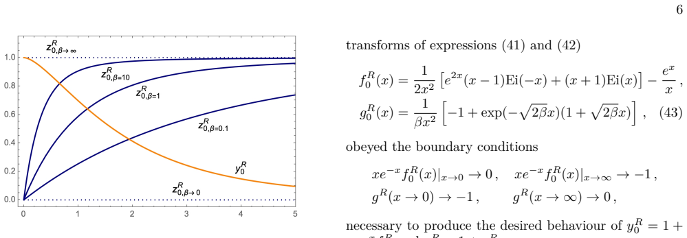
Laplace-plane expansion in thef R,g R coordinates In terms offR andg R defined by Eqs. (26) and (27), theODEsystem(1)-(2)canberewrittenintheschematic form Lf B[fR] = ex x +e−2x(fR)3 + 3e−x(fR)2 x (28) + ( fR + ex x ) gR(2 +gR), Lg B[gR] = 2e−2x(gR + 1) ( fR + ex x )2 (29) +β(gR)2(gR + 3), where the linear operators on the LHS’s read Lf B[f](x)≡f′′(x)−2f′(...
-
[6]
global backgrounds
Borel-plane calculation of ˆfR 0 ,ˆgR 0 Due to the rather special shape of the linear oper- ators (30) that differ from those of Eq. (19) in the 1/x2-proportional pieces, the Borel-plane counterparts of Eqs. (28), (29) assume particularly nice forms (with the genericˆrf,ˆrg symbols denoting the relevant RHS expres- sions) t(t+ 2) ˆfR(t) + ∫ t 0 dsKf B(t,s...
-
[7]
The two offsets Hence, in what follows, the central quantities of our interest will be theoffsetsof the gauge/vector and scalar profiles from 1 defined by y(x) = 1 +v(x),(46) z(x) = 1 +s(x). In the scalar sector,sis just a (natural) relabelling of gand/org R used in Sects IIA and IIB and also in Ref.[7], whilev(x) =xe −xfR(x)representsanewcoordi- nate str...
-
[8]
,(51) s=s 0 +s 1 +s 2 +
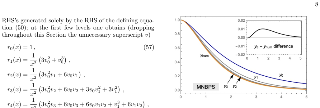
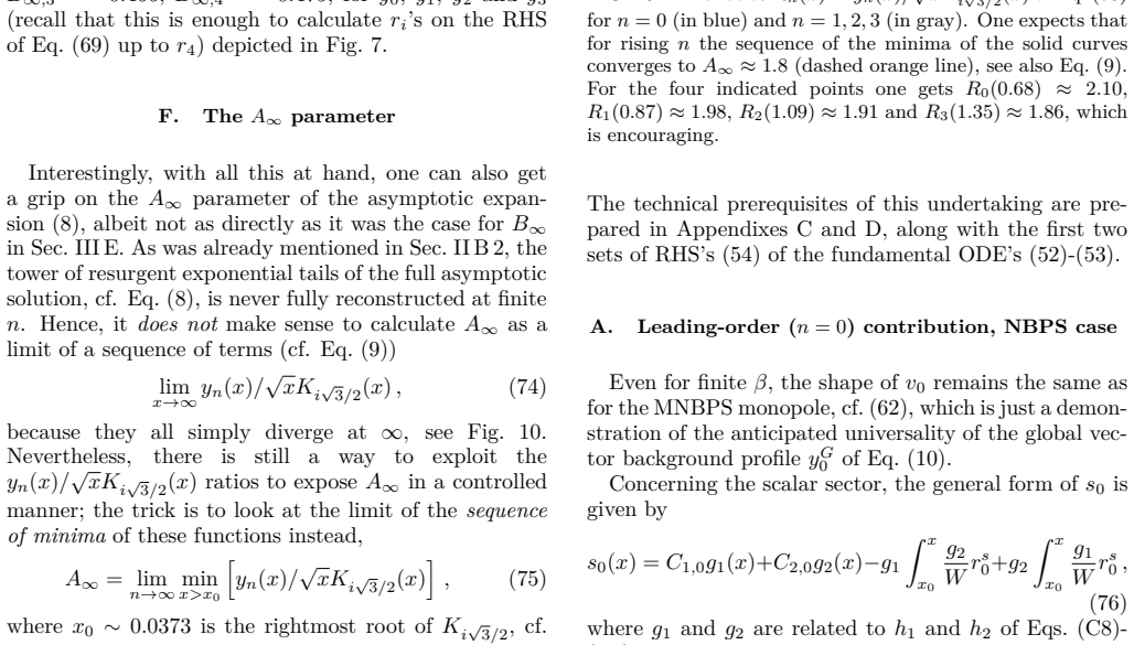
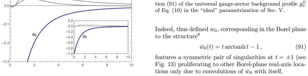
The triangular expansion A natural triangular perturbative scheme then emerges from the expansion v=v 0 +v 1 +v 2 +... ,(51) s=s 0 +s 1 +s 2 +... , which, substituted into Eqs. (47)-(48) yields a tower of ODE’s for the individual levelsvn ands n, v′′ n− ( 1 + 2 x2 ) vn =r v n,(52) s′′ n + 2s′ n x − ( 2β+ 2 x2 ) sn =r s n,(53) with completely universal LHS...
-
[9]
seed element
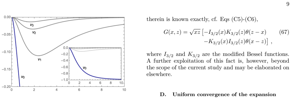
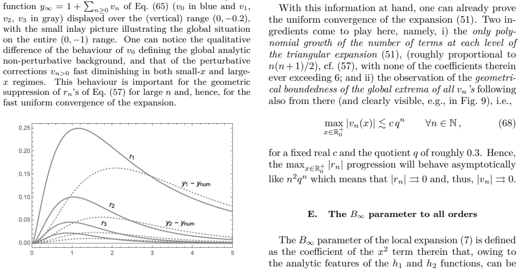
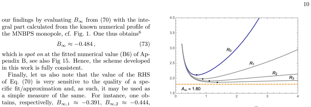
+ 2 x2v0(2 +v 0)(1 +s 0), and so on3. In parametrization (46), the boundary con- ditions (4)-(5) translate into v0(x→0)→0, v0(x→∞)→−1,(55) vn(x→0)→0, vn(x→∞)→0,forn>0, and s0(x→0)→−1, s0(x→∞)→0,(56) sn(x→0)→0, s n(x→∞)→0,forn>0. Note that, for each leveln, ther v,s n structures on the RHS’s of Eqs. (52)-(53) are fixed and known as they are constructed sol...
-
[10]
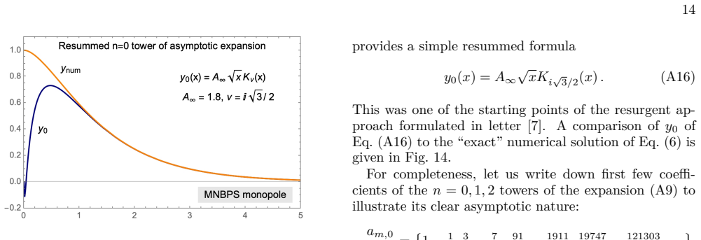
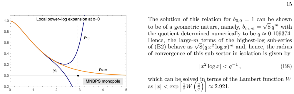
14: Comparison of the resummed leading asymptotic (gauge) profile of the MNBPS monopoley0 of Eq
= ∞∑ m=0 dmzm,(A7) where dm = 1 C cm,1 m! .(A8) Borel resummation of then= 0tower Thisallmeansthattheexpansion(A1)wehavestarted with can be eventually written as y(x) = ∞∑ m=0 m∑ n=0 am,nx−me−(2n+1)x,(A9) 14 FIG. 14: Comparison of the resummed leading asymptotic (gauge) profile of the MNBPS monopoley0 of Eq. (A16) (in blue) to the “exact” numerical soluti...
1911
-
[11]
canonical pair
Laplace-plane viewpoint The general solution of Eq. (C1) can be written as v(x) =h(x) +p(x),(C2) wherehis the solution to its homogeneous version h′′(x)− ( 1 + 2 x2 ) h(x) = 0,(C3) andpis the particular solution associated tor(x), ob- tained by the variation of constants method. a. Homogeneous solution As for the homogeneous part, employingh(x)≡√xa(x), Eq...
-
[12]
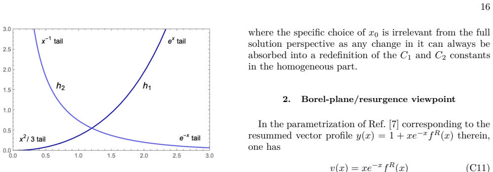
optically
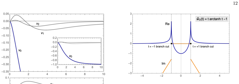
Borel-plane/resurgence viewpoint In the parametrization of Ref. [7] corresponding to the resummed vector profiley(x) = 1 +xe −xfR(x)therein, one has v(x) =xe−xfR(x)(C11) and, thus, the Borel-plane equivalent of the ODE (C1) written in terms ofˆfR reads t(t+ 2) ˆfR(t)−2(t+ 1) ∫ t 0 ds ˆfR(s) = ˆrf(t),(C12) withˆrf(t)denoting the Borel-plane representation ...
-
[13]
Laplace-plane viewpoint As before, we write the general solution to Eq. (D1) in terms of the homogeneous and particular solutions, s(x) =h(x) +p(x),(D2) wherehis the general solution of s′′(x) + 2s′(x) x − ( 2β+ 2 x2 ) s(x) = 0,(D3) andpassociated to a non-zero RHS of Eq. (D1) is ob- tained as usual by variation of its constants. a. Homogeneous solution H...
-
[14]
Dirac comb
Borel-plane/resurgence viewpoint The Volterra equation equivalent to Eq. (D1) reads (t2−2β)ˆs(t)−2t ∫ t 0 dzˆs(z) = ˆrs(t),(D8) whereˆrs(t)is the Borel-plane equivalent ofr(x)therein. Note that this Equation has two singularities att= ±√2β. Again, the two integrals corresponding to the 2s′(x)/xand−2s(x)/x2 structures in Eq. (D1) combine in such a way to p...
-
[15]
Georgi and S
H. Georgi and S. L. Glashow, Phys. Rev. Lett.32, 438 (1974)
1974
-
[16]
’t Hooft, Nucl
G. ’t Hooft, Nucl. Phys. B79, 276 (1974)
1974
-
[17]
A. M. Polyakov, JETP Lett.20, 194 (1974)
1974
-
[18]
J. A. Bryan, S. M. Carroll, and T. Pyne, Phys. Rev. D 50, 2806 (1994)
1994
-
[19]
M. K. Prasad and C. M. Sommerfield, Phys. Rev. Lett. 35, 760 (1975)
1975
-
[20]
E. B. Bogomolny, Sov. J. Nucl. Phys.24, 449 (1976)
1976
- [21]
-
[22]
Julia and A
B. Julia and A. Zee, Phys. Rev. D11, 2227 (1975)
1975
-
[23]
F. A. Bais and J. R. Primack, Phys. Rev. D13, 819 (1976)
1976
-
[24]
Goddard and D
P. Goddard and D. I. Olive, Rept. Prog. Phys.41, 1357 (1978)
1978
-
[25]
C. L. Gardner, Annals of Physics146, 129 (1983)
1983
-
[26]
Breitenlohner, P
P. Breitenlohner, P. Forgács, and D. Maison, Nuclear Physics B383, 357 (1992)
1992
-
[27]
P. Forgacs, N. Obadia, and S. Reuillon, Phys. Rev. D71, 035002 (2005), arXiv:hep-th/0412057, [Erratum: Phys.Rev.D 71, 119902 (2005)]
Pith/arXiv arXiv 2005
-
[28]
G. V. Dunne and E. Shinn, arXiv:2602.17583
-
[29]
Écalle,Les fonctions resurgentes; Vols
J. Écalle,Les fonctions resurgentes; Vols. 1-3(Prépub. Math. Univ. Paris-Sud 81-05 (1981), 81-06 (1981), 85-05 (1985))
1981
-
[30]
B. J. Sternin and V. E. Shatalov,Borel-Laplace trans- form and asymptotic theory : introduction to resurgent analysis(CRC Press, Boca Raton, FL, 1996)
1996
-
[31]
Costin,Asymptotics and Borel Summability(Chap- man and Hall/CRC, 2008, ISBN: 1420070312)
O. Costin,Asymptotics and Borel Summability(Chap- man and Hall/CRC, 2008, ISBN: 1420070312)
2008
-
[32]
I. Aniceto, R. Schiappa, and M. Vonk, Commun. Num. Theor. Phys.6, 339 (2012), arXiv:1106.5922
Pith/arXiv arXiv 2012
-
[33]
G. V. Dunne and M. Ünsal, Phys. Rev. D89, 041701 (2014), arXiv:1306.4405
Pith/arXiv arXiv 2014
-
[34]
Mariño, An introduction to resurgence in quantum theory, Lecture notes available at https://www.marcosmarino.net/uploads/1/3/3/5/ 133535336/resurgence-course.pdf
M. Mariño, An introduction to resurgence in quantum theory, Lecture notes available at https://www.marcosmarino.net/uploads/1/3/3/5/ 133535336/resurgence-course.pdf
-
[35]
I. Aniceto and R. Schiappa, Commun. Math. Phys.335, 183 (2015), arXiv:1308.1115
Pith/arXiv arXiv 2015
-
[36]
Dorigoni, Annals Phys.409, 167914 (2019), arXiv:1411.3585
D. Dorigoni, Annals Phys.409, 167914 (2019), arXiv:1411.3585
arXiv 2019
-
[37]
Mitschi, D
C. Mitschi, D. Sauzin, E. Delabaere, and M. Loday- Richaud,Divergent Series, Summability and Resurgence I-III(Springer 2017, Volumes 2153-2155)
2017
-
[38]
I. Aniceto, G. Basar, and R. Schiappa, Phys. Rept.809, 1 (2019), arXiv:1802.10441
arXiv 2019
-
[39]
G. V. Dunne, arXiv:2511.15528
discussion (0)
Sign in with ORCID, Apple, or X to comment. Anyone can read and Pith papers without signing in.