Numerical self-force calculations for scalar particles, formulated in the lab frame
Pith reviewed 2026-06-27 23:53 UTC · model grok-4.3
The pith
Scalar self-force equations derived in the lab frame with finite particle size h simplify and become directly suitable for numerical discretization.
A machine-rendered reading of the paper's core claim, the machinery that carries it, and where it could break.
Core claim
By assuming a small but finite discretization length scale h, choosing the state vector for the system before deriving equations of motion, and formulating the equations explicitly in the lab frame, the authors obtain self-consistent equations of motion for scalar particles interacting with a scalar field. This approach greatly simplifies the resulting equations and their derivation while remaining directly suitable for numerical calculations via an effective source method. The method is illustrated with two possible discretizations based on finite volumes and spectral methods; one-dimensional calculations exhibit excellent agreement with analytic solutions.
What carries the argument
The lab-frame effective source method constructed with finite discretization length h, which treats the particle as a small finite object and carries the simplification of the equations.
If this is right
- The equations admit direct discretization by finite-volume or spectral methods.
- One-dimensional implementations agree with analytic solutions to high accuracy.
- The effective source construction extends straightforwardly to electrodynamics and general relativity.
- Self-force effects that include radiation reaction are captured without additional regularization steps.
Where Pith is reading between the lines
- The lab-frame starting point may reduce the need for coordinate transformations when the same method is applied inside existing Cartesian numerical codes.
- Testing the same construction for a particle on a circular orbit in Schwarzschild spacetime would check whether the reported simplification survives curvature.
- The finite-h regularization might be compared directly with other point-particle regularizations to measure any difference in the extracted self-force.
Load-bearing premise
That selecting the state vector before deriving the equations and writing them in the lab frame rather than covariantly produces a self-consistent simplification that remains accurate when h is taken small but finite.
What would settle it
A numerical solution of the discretized equations in a known analytic self-force problem that deviates from the exact radiation-reaction force when h is reduced would show the approach fails to remain accurate.
Figures


read the original abstract
We derive equations of motion for scalar particles self-consistently interacting with a scalar field,including the radiation produced by the particles' acceleration. Our approach differs in three key aspects from current methods: (1) we assume a small but finite discretization length scale $h$, which allows us to treat the particle as a small but finite object, (2) we choose the state vector for the system before deriving equations of motion, and (3) we formulate the equations explicitly in the lab frame and not in a manifestly covariant manner. This approach, which is self-consistent, happens to greatly simplify the resulting equations and their derivation, and is directly suitable for numerical calculations. The result is an effective source method which generalizes to electrodynamics or general relativity in a straightforward manner (although we do not consider this here). We then provide two possible discretizations of these equations, based on finite volumes and spectral methods, and show results of one-dimensional calculations. These calculations show excellent agreement with analytic solutions.
Editorial analysis
A structured set of objections, weighed in public.
Referee Report
Summary. The paper derives equations of motion for scalar particles self-consistently interacting with a scalar field by assuming a small but finite discretization length h, selecting the state vector prior to deriving the equations, and formulating everything explicitly in the lab frame rather than in a manifestly covariant way. This produces an effective-source formulation that the authors state greatly simplifies the equations and is directly amenable to numerical discretization. Finite-volume and spectral discretizations are presented, with one-dimensional numerical results shown to agree with known analytic solutions to high accuracy. Generalization to electrodynamics or general relativity is asserted to be straightforward but is not carried out.
Significance. If the central claims hold, the lab-frame finite-h approach offers a numerically practical route to self-force calculations for the scalar case, with the 1D agreement to analytic solutions providing concrete evidence of self-consistency and implementability. The explicit choice of state vector and avoidance of manifest covariance are presented as sources of simplification; if these survive detailed scrutiny they could reduce the technical overhead of effective-source methods.
major comments (2)
- [Abstract] Abstract and the paragraph on the three key aspects: the claim that the approach 'greatly simplifies the resulting equations and their derivation' rests on a derivation that is summarized rather than exhibited in full; without the explicit steps showing how the lab-frame state-vector choice eliminates terms or yields the effective source, it is difficult to assess whether the simplification is genuine or merely a re-arrangement.
- [Numerical results] The numerical section (1D calculations): while agreement with analytic solutions is reported, the manuscript does not quantify the dependence on the free parameter h (e.g., convergence rate as h is reduced while remaining finite) or demonstrate that the physical solution is recovered in the h o0 limit; this is load-bearing for the assertion that finite but small h remains physically accurate.
minor comments (2)
- Notation for the state vector and the effective source should be introduced with an explicit definition before first use to improve readability for readers unfamiliar with the lab-frame formulation.
- The manuscript would benefit from a short table comparing the number of terms or the structure of the equations obtained here versus a standard covariant effective-source derivation, even if only schematic.
Simulated Author's Rebuttal
We thank the referee for their careful reading of the manuscript and for the constructive comments. We address the two major points below and indicate the revisions that will be incorporated.
read point-by-point responses
-
Referee: [Abstract] Abstract and the paragraph on the three key aspects: the claim that the approach 'greatly simplifies the resulting equations and their derivation' rests on a derivation that is summarized rather than exhibited in full; without the explicit steps showing how the lab-frame state-vector choice eliminates terms or yields the effective source, it is difficult to assess whether the simplification is genuine or merely a re-arrangement.
Authors: We agree that the derivation steps are presented in summarized form and that additional explicit detail would allow readers to evaluate the claimed simplification directly. In the revised manuscript we will expand the derivation section to exhibit the intermediate steps, showing how the pre-chosen lab-frame state vector removes specific terms and produces the effective source. revision: yes
-
Referee: [Numerical results] The numerical section (1D calculations): while agreement with analytic solutions is reported, the manuscript does not quantify the dependence on the free parameter h (e.g., convergence rate as h is reduced while remaining finite) or demonstrate that the physical solution is recovered in the h→0 limit; this is load-bearing for the assertion that finite but small h remains physically accurate.
Authors: The existing 1D results demonstrate agreement at a fixed small but finite h. We acknowledge that a quantitative study of the h-dependence is needed to support the physical accuracy claim. We will add a new subsection (or supplementary figure) that varies h, reports the observed convergence rate, and explicitly shows recovery of the analytic solution as h approaches zero. revision: yes
Circularity Check
No significant circularity
full rationale
The derivation begins from explicit assumptions (finite h, chosen state vector, lab-frame formulation) and produces effective-source equations that are then discretized and validated against independent analytic solutions in 1D. No step reduces a claimed prediction or result to a fitted parameter, self-definition, or load-bearing self-citation chain. The generalization claim is explicitly scoped as future work and not used to support the scalar results. The central claims remain independent of the paper's own outputs.
Axiom & Free-Parameter Ledger
free parameters (1)
- h
axioms (1)
- standard math Scalar field equations govern the particle-field interaction
Forward citations
Cited by 1 Pith paper
-
Self-force on a static scalar charge in traversable wormholes
Mode-sum computation of static scalar self-force in Konoplya-Zhidenko wormholes shows parameter-dependent sign changes and slower-than-usual large-distance decay for large redshift parameter p.
Reference graph
Works this paper leans on
-
[1]
As described above, we assume thatρ 0 has a finite support of sizeℓ, withℓ≲hwherehis a given length cutoff parameter
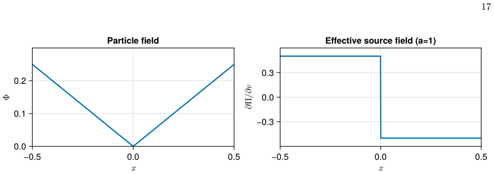
Particle at rest We define the charge distribution for a particle at rest at the origin to beρ 0(xi). As described above, we assume thatρ 0 has a finite support of sizeℓ, withℓ≲hwherehis a given length cutoff parameter. 4 This charge distribution is associated with a scalar field Φ 0(xi) through the Poisson equation δij∂i∂jΦ0 :=ρ 0 . (4) This particle has...
-
[2]
We describe the particle at a fixed instance of time in the lab frame
Moving particle We consider a particle located at positionz i and moving with a constant three-velocityv i. We describe the particle at a fixed instance of time in the lab frame. This will allow us below to make the particle part of the state vector; a state vector describes a physical system at an instance of time. The charge distribution and potential a...
-
[3]
at rest at that instant in time
Zeno’s Arrow Paradox In the arrow paradox [37, 38], Zeno of Elea (c. 490–430 BC) argues: . . . If everything when it occupies an equal space is at rest at that instant of time, and if that which is in locomotion is always occupying such a space at any moment, the flying arrow is therefore motionless at that instant of time and at the next instant of time ...
-
[4]
Particle equations of motion We describe the particle trajectory by the functionsz i p(t) andv i p(t). The well-known equations of motion for the particle in a given external (background) potential Φ e are then ∂tzi p =v i p (18) γ(M 0 +QΦ e)∂ tvi p ≈ −Qδ ij∂jΦe(zi p) (19) with the particle charge distribution ρp(t, xi) :=ρ lab(zi p(t), vi p(t);x i).(20) ...
-
[5]
Representing the particle field We choose to define the particle field Φ p (at a timet) as the field of a non-accelerating particle (at that same time t), as seen in the lab frame. We already defined these quantities in section III B 2 above: Φp(t, xi) := Φ lab(zi p(t), vi p(t);x i) (24) Πp(t, xi) := Π lab(zi p(t), vi p(t);x i) (25) ρp(t, xi) :=ρ lab(zi p...
-
[6]
one dimension
Equations of motion The equations of motion for the remainder fields Φ r and Πr are now automatically also defined. They follow from the equations of motion for the physical fields Φ and Π. They are ∂tΦr =∂ tΦ−∂ tΦp (36) = Π−Π p −S Φ (37) = Π r −S Φ (38) ∂tΠr =∂ tΠ−∂ tΠp (39) =δ ij∂i∂jΦ−ρ−δ ij∂i∂jΦp +ρ p −S Π (40) =δ ij∂i∂jΦr −S Π (41) These are the same ...
-
[7]
First-order formulation We rewrite the system (36) above in a fully first-order form by introducing a new variable Ψ i :=∂ iΦ: ∂tΦr = Π r −S Φ (42) ∂tΠr =δ ij∂iΨr,j −S Π (43) ∂tΨr,i =∂ iΠr −S Ψ (44) where SΨ :=∂ iSΦ . (45)
-
[8]
Characteristics We represent the field equations as a first-order hyperbolic system. We define the field state-vectorU f and the evolution system as: ∂t ¯Uf +A∂ x ¯Uf =S(46) where Uf = Πr Ψr Φr , A= 0−1 0 −1 0 0 0 0 0 , S= −ai∂viΠlab −ai∂viΨlab −ai∂viΦlab ,(47) whereU f is the field part of the state-vector,Ais the principal part a...
-
[9]
We employ a staggered grid where thei-th cell is defined by the interval Ωi = (xi−1/2, xi+1/2).(51) wherex i±1/2 =x i ±h/2
Computational grid We discretize the spatial domain [−L, L] intoNcells of widthh. We employ a staggered grid where thei-th cell is defined by the interval Ωi = (xi−1/2, xi+1/2).(51) wherex i±1/2 =x i ±h/2. The discrete variable ¯U n i describes the average value ¯U n i = 1 h Z Ωi U(t n, x) dx.(52) By working with cell averages we can ensure the numerical ...
-
[10]
Weak formulation Since (46) contains low regularity source terms, we interpret the evolution in a weak sense. Specifically, we require the residual of the evolution equation to be orthogonal to our basis functionsb i(x): ⟨∂tU+∂ x(AU)−S, b i⟩= 0.(57) Expanding the inner product using the definition ofb i(x) yields: Z Ωi ∂tUdx+ Z Ωi ∂x(AU) dx= Z Ωi Sdx.(58)...
-
[11]
Numerical fluxes Since the flux calculations are being performed at the cell faces, we need to introduce a numerical flux to approximate the fluxes at the faces based on the values ofUat the cell centers. We use the Godunov flux [50], which is the same 10 as the Rusanov flux [57] for the linear wave equation, since the local Lax-Friedrichs speed [58] is g...
-
[12]
These methods are also known as Monotonic Upstream-centered Scheme for Conservation Laws (MUSCL) [59, 60]
Second-order approximation To resolve discontinuous data at second order, a standard practice is to employ slope limiters and linear reconstruc- tion in characteristic space. These methods are also known as Monotonic Upstream-centered Scheme for Conservation Laws (MUSCL) [59, 60]. The homogeneous part is thus ensured to be Total Variation Diminishing (TVD...
-
[13]
The source contribution is computed ana- lytically by evaluating the cell-averaging integral over each computational cell
Source treatment We employ an unsplit method for the time evolution of the field equations, wherein the source term is incorporated directly into the right-hand side of the homogeneous evolution equations. The source contribution is computed ana- lytically by evaluating the cell-averaging integral over each computational cell. To accurately capture the be...
-
[14]
smearing
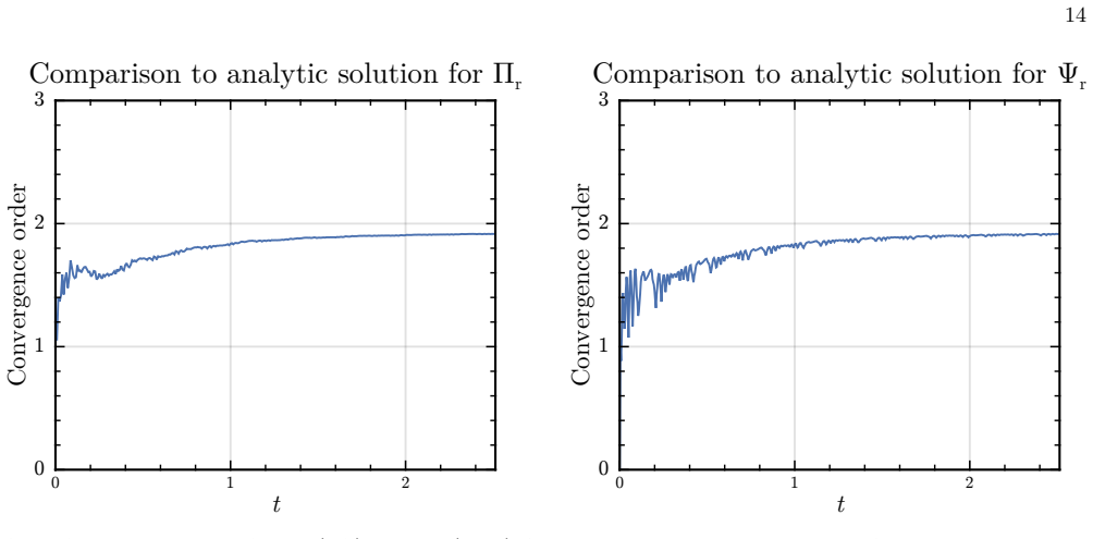
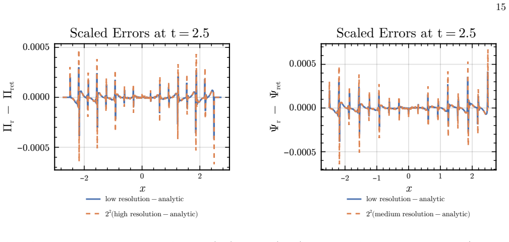
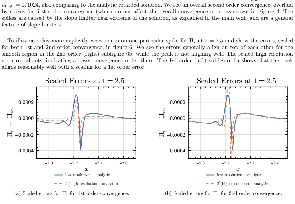
Convergence analysis While smooth solutions allow for pointwise convergence analysis in theL∞ (max) norm, discontinuous data typically undergoes “smearing” over a few grid cells due to numerical diffusion. In such cases, the error at the jump does not decrease in the infinity norm regardless of the grid refinement. Therefore, we quantify convergence using...
-
[15]
We do this exactly, summing the spectral basis functions and their derivatives
We evaluate the fields Φr and Πr and their gradients at the particle positionz. We do this exactly, summing the spectral basis functions and their derivatives. We then evaluate the terms in the particle’s equations of motion (18). We also add a forcing term for some test cases (see below)
-
[16]
spectrally
We apply the Laplace operator to Φ n r . Since we already calculated the particle accelerationa=d/dt vwe can evaluate the source terms at each Gauss-Legendre quadrature node. This allows us to explicitly project the source terms onto each basis function, filtering out all high-frequency noise. It well known that specral methods converge “spectrally” (esse...
-
[17]
approximately corrected for radiation
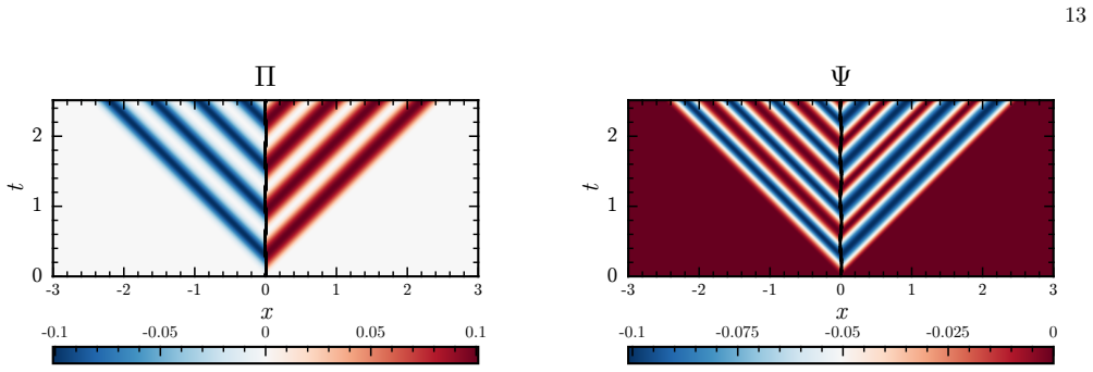
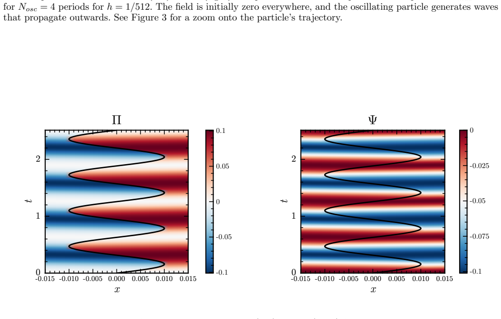
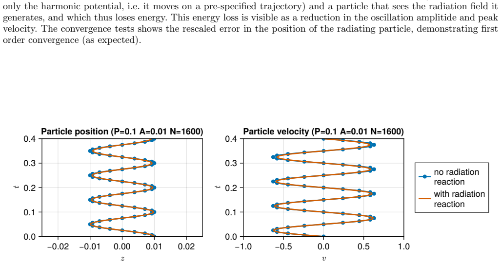
Forced motion We simulate a particle with chargeq= 1 that oscillates with maximum velocityv max = 0.1 and amplitudeA= 0.01. We evolve for a total timet f = 2.5 during which the particle oscillate 4 times, thus we choose the domain [−L, L] with L= 6. This domain size is chosen specifically so that, during the time frame of the four oscillations, any numeri...
-
[18]
P. A. M. Dirac, Classical theory of radiating electrons, Proc. Roy. Soc. Lond. A167, 148 (1938)
1938
-
[19]
B. S. DeWitt and R. W. Brehme, Radiation damping in a gravitational field, Annals Phys.9, 220 (1960)
1960
-
[20]
Y. Mino, M. Sasaki, and T. Tanaka, Gravitational radiation reaction to a particle motion, Phys. Rev. D55, 3457 (1997)
1997
-
[21]
T. C. Quinn and R. M. Wald, An axiomatic approach to electromagnetic and gravitational radiation reaction of particles in curved space-time, Phys. Rev. D56, 3381 (1997)
1997
-
[22]
Detweiler and B
S. Detweiler and B. F. Whiting, Self-force via a green’s function decomposition, Phys. Rev. D67, 024025 (2003)
2003
-
[23]
S. E. Gralla and R. M. Wald, A rigorous derivation of gravitational self-force, Class. Quant. Grav.25, 205009 (2008)
2008
-
[24]
Pound, Self-consistent gravitational self-force, Phys
A. Pound, Self-consistent gravitational self-force, Phys. Rev. D81, 024023 (2010)
2010
-
[25]
Rosenthal, Regularization of the second-order gravitational perturbations produced by a compact object, Phys
E. Rosenthal, Regularization of the second-order gravitational perturbations produced by a compact object, Phys. Rev. D 72, 121503 (2005)
2005
-
[26]
Rosenthal, Second-order gravitational self-force, Phys
E. Rosenthal, Second-order gravitational self-force, Phys. Rev. D74, 084018 (2006)
2006
-
[27]
Pound, Second-order gravitational self-force, Phys
A. Pound, Second-order gravitational self-force, Phys. Rev. Lett.109, 051101 (2012)
2012
-
[28]
S. E. Gralla, Second order gravitational self force, Phys. Rev. D85, 124011 (2012)
2012
-
[29]
Detweiler, Gravitational radiation reaction and second order perturbation theory, Phys
S. Detweiler, Gravitational radiation reaction and second order perturbation theory, Phys. Rev. D85, 044048 (2012)
2012
-
[30]
Poisson, A
E. Poisson, A. Pound, and I. Vega, The motion of point particles in curved spacetime, Living Reviews in Relativity14, 7 (2011)
2011
-
[31]
Detweiler, Perspective on gravitational self-force analyses, Classical and Quantum Gravity22, S681 (2005)
S. Detweiler, Perspective on gravitational self-force analyses, Classical and Quantum Gravity22, S681 (2005)
2005
-
[32]
Barack, Gravitational self-force in extreme mass-ratio inspirals, Classical and Quantum Gravity26, 213001 (2009)
L. Barack, Gravitational self-force in extreme mass-ratio inspirals, Classical and Quantum Gravity26, 213001 (2009)
2009
-
[33]
Blanchet, A
L. Blanchet, A. Spallicci, and B. Whiting, eds.,Mass and motion in general relativity. Proceedings, School on Mass, Orleans, France, June 23-25, 2008, Vol. 162 (Springer, Dordrecht, 2011)
2008
-
[34]
Mino, Perturbative approach to an orbital evolution around a supermassive black hole, Phys
Y. Mino, Perturbative approach to an orbital evolution around a supermassive black hole, Phys. Rev. D67, 084027 (2003)
2003
-
[35]
S. A. Hughes, S. Drasco, E. E. Flanagan, and J. Franklin, Gravitational radiation reaction and inspiral waveforms in the adiabatic limit, Phys. Rev. Lett.94, 221101 (2005)
2005
-
[36]
Drasco and S
S. Drasco and S. A. Hughes, Gravitational wave snapshots of generic extreme mass ratio inspirals, Phys. Rev. D73, 024027 (2006)
2006
-
[37]
P. A. Sundararajan, G. Khanna, and S. A. Hughes, Towards adiabatic waveforms for inspiral into kerr black holes. i. a new model of the source for the time domain perturbation equation, Phys. Rev. D76, 104005 (2007)
2007
-
[38]
Barack and A
L. Barack and A. Ori, Mode sum regularization approach for the self-force in black hole space-time, Phys. Rev. D61, 061502 (2000)
2000
-
[39]
Barack, Y
L. Barack, Y. Mino, H. Nakano, A. Ori, and M. Sasaki, Calculating the gravitational self-force in schwarzschild space-time, Phys. Rev. Lett.88, 091101 (2002)
2002
-
[40]
Poisson and A
E. Poisson and A. G. Wiseman, Suggestion at the 1st capra ranch meeting on radiation reaction (1998)
1998
-
[41]
W. G. Anderson and A. G. Wiseman, A matched expansion approach to practical self-force calculations, Class. Quant. Grav.22, S783 (2005)
2005
-
[42]
Casals, S
M. Casals, S. Dolan, A. C. Ottewill, and B. Wardell, Self-force and green function in schwarzschild spacetime via quasi- normal modes and branch cut, Phys. Rev. D88, 044022 (2013). 22
2013
-
[43]
Wardell, C
B. Wardell, C. R. Galley, A. Zenginoglu, M. Casals, S. R. Dolan, and A. C. Ottewill, Self-force via green functions and worldline integration, Phys. Rev. D89, 084021 (2014)
2014
-
[44]
Zenginoglu and C
A. Zenginoglu and C. R. Galley, Caustic echoes from a schwarzschild black hole, Phys. Rev. D86, 064030 (2012)
2012
-
[45]
Barack and D
L. Barack and D. A. Golbourn, Scalar-field perturbations from a particle orbiting a black hole using numerical evolution in 2+1 dimensions, Phys. Rev. D76, 044020 (2007)
2007
-
[46]
Vega and S
I. Vega and S. Detweiler, Regularization of fields for self-force problems in curved spacetime: Foundations and a time-domain application, Phys. Rev. D77, 084008 (2008)
2008
-
[47]
S. R. Dolan and L. Barack, Self force via m-mode regularization and 2+1d evolution: Foundations and a scalar-field implementation on schwarzschild, Phys. Rev. D83, 024019 (2011)
2011
-
[48]
Diener, I
P. Diener, I. Vega, B. Wardell, and S. Detweiler, Self-consistent orbital evolution of a particle around a schwarzschild black hole, Phys. Rev. Lett.108, 191102 (2012)
2012
-
[49]
Warburton and B
N. Warburton and B. Wardell, Applying the effective-source approach to frequency-domain self-force calculations, Phys. Rev. D89, 044046 (2014)
2014
-
[50]
Heffernan, A
A. Heffernan, A. C. Ottewill, N. Warburton, B. Wardell, and P. Diener, Accelerated motion and the self-force in schwarzschild spacetime, Classical and Quantum Gravity35, 194001 (2018)
2018
-
[51]
Advances and Challenges in Computational Relativity
P. Diener, Challenges in the self-consistent evolution of extreme mass ratio inspirals, Talk presented at the ICERM Workshop “Advances and Challenges in Computational Relativity” (2020), september 16, 2020; in collaboration with Barry Wardell and Niels Warburton
2020
-
[52]
N. A. Wittek, A. Pound, H. P. Pfeiffer, and L. Barack, Worldtube excision method for intermediate-mass-ratio inspirals: Self-consistent evolution in a scalar-charge model, Phys. Rev. D110, 084023 (2024)
2024
-
[53]
N. A. Wittek, L. Barack, H. P. Pfeiffer, A. Pound, N. Deppe, L. E. Kidder, A. Macedo, K. C. Nelli, W. Throwe, and N. L. Vu, Relieving scale disparity in binary black hole simulations, Phys. Rev. Lett.134, 251402 (2025)
2025
-
[54]
H. D. P. Lee,Zeno of Elea(Cambridge University Press, 2015)
2015
-
[55]
Vlastos, A note on zeno’s arrow, Phronesis11, 3 (1966)
G. Vlastos, A note on zeno’s arrow, Phronesis11, 3 (1966)
1966
-
[56]
Huggett, Zeno’s Paradoxes, inThe Stanford Encyclopedia of Philosophy, edited by E
N. Huggett, Zeno’s Paradoxes, inThe Stanford Encyclopedia of Philosophy, edited by E. N. Zalta and U. Nodelman (Metaphysics Research Lab, Stanford University, 2025) Winter 2025 ed
2025
-
[57]
Laertius,Lives of Eminent Philosophers, Volume I: Books 1-5, Loeb Classical Library, Vol
D. Laertius,Lives of Eminent Philosophers, Volume I: Books 1-5, Loeb Classical Library, Vol. 184 (Harvard University Press, Cambridge, MA, 1925)
1925
-
[58]
Barack and A
L. Barack and A. Pound, Self-force and radiation reaction in general relativity, Reports on Progress in Physics82, 016904 (2018)
2018
-
[59]
I. Vega, P. Diener, W. Tichy, and S. Detweiler, Self-force with (3 + 1) codes: A primer for numerical relativists, Phys. Rev. D80, 084021 (2009)
2009
-
[60]
Heffernan, A
A. Heffernan, A. Ottewill, and B. Wardell, High-order expansions of the detweiler-whiting singular field in schwarzschild spacetime, Phys. Rev. D86, 104023 (2012)
2012
-
[61]
Detweiler, E
S. Detweiler, E. Messaritaki, and B. F. Whiting, Self-force of a scalar field for circular orbits about a schwarzschild black hole, Phys. Rev. D67, 104016 (2003)
2003
-
[62]
I. Vega, B. Wardell, and P. Diener, Effective source approach to self-force calculations, Classical and Quantum Gravity 28, 134010 (2011)
2011
-
[63]
Bourg, A
P. Bourg, A. Pound, S. D. Upton, and R. P. Macedo, Simple, efficient method of calculating the detweiler-whiting singular field to very high order, Phys. Rev. D110, 084007 (2024)
2024
-
[64]
Heffernan, A
A. Heffernan, A. Ottewill, and B. Wardell, High-order expansions of the detweiler-whiting singular field in kerr spacetime, Phys. Rev. D89, 024030 (2014)
2014
-
[65]
Wardell, I
B. Wardell, I. Vega, J. Thornburg, and P. Diener, Generic effective source for scalar self-force calculations, Phys. Rev. D 85, 104044 (2012)
2012
-
[66]
R. J. LeVeque,Finite Volume Methods for Hyperbolic Problems, Cambridge Texts in Applied Mathematics (Cambridge University Press, 2002)
2002
-
[67]
S. K. Godunov, A difference method for numerical calculation of discontinuous solutions of the equations of hydrodynamics, Matematicheskii Sbornik47, 271 (1959), original Russian title:Raznostnyi metod chislennogo rascheta razryvnykh reshenii uravnenii gidrodinamiki
1959
-
[68]
W. E. Schiesser,The Numerical Method of Lines: Integration of Partial Differential Equations(Elsevier Science, 2012)
2012
-
[69]
S. J. Ruuth, Global optimization of explicit strong-stability-preserving runge-kutta methods, Mathematics of Computation 75, 183 (2006)
2006
-
[70]
B. A. Finlayson,The Method of Weighted Residuals and Variational Principles(Society for Industrial and Applied Math- ematics, Philadelphia, PA, 2013) https://epubs.siam.org/doi/pdf/10.1137/1.9781611973242
-
[71]
I. G. Bubnov, Report on the works of professor timoshenko which were awarded the zhuranskyi prize, inSymposium of the institute of communication engineers, Vol. 81 (1913)
1913
-
[72]
B. G. Galerkin, Series solution of some problems of elastic equilibrium of rods and plates, Vestnik inzhenerov i tekhnikov 19, 897 (1915)
1915
-
[73]
Petrov, Application of galerkin’s method to the problem of stability of flow of a viscous fluid, J
G. Petrov, Application of galerkin’s method to the problem of stability of flow of a viscous fluid, J. Appl. Math. Mech4, 3 (1940)
1940
-
[74]
Rusanov, The calculation of the interaction of non-stationary shock waves and obstacles, USSR Computational Math- ematics and Mathematical Physics1, 304 (1962)
V. Rusanov, The calculation of the interaction of non-stationary shock waves and obstacles, USSR Computational Math- ematics and Mathematical Physics1, 304 (1962)
1962
-
[75]
K. O. Friedrichs and P. D. Lax, Systems of conservation equations with a convex extension, Proceedings of the National Academy of Sciences68, 1686 (1971), https://www.pnas.org/doi/pdf/10.1073/pnas.68.8.1686. 23
-
[76]
Van Leer, Towards the ultimate conservative difference scheme
B. Van Leer, Towards the ultimate conservative difference scheme. IV. A new approach to numerical convection, Journal of Computational Physics23, 276 (1977)
1977
-
[77]
van Leer, Towards the ultimate conservative difference scheme
B. van Leer, Towards the ultimate conservative difference scheme. v. a second-order sequel to godunov’s method, Journal of Computational Physics32, 101 (1979)
1979
-
[78]
Harten, High resolution schemes for hyperbolic conservation laws, Journal of Computational Physics49, 357 (1983)
A. Harten, High resolution schemes for hyperbolic conservation laws, Journal of Computational Physics49, 357 (1983)
1983
-
[79]
FastGaussQuadrature.jl Julia package (2025),https://github.com/JuliaApproximation/FastGaussQuadrature.jl
2025
discussion (0)
Sign in with ORCID, Apple, or X to comment. Anyone can read and Pith papers without signing in.