REVIEW 2 major objections 6 minor 68 references
JAX-FEM-ANISO: Differentiable GPU-Accelerated Finite Element Framework for Inverse Identification of Finite-Strain Anisotropic Plasticity
T0 review · 2 major / 6 minor · reviewed 2026-07-14 · grok-4.5
Pith's one-line read A GPU-differentiable finite-element code recovers anisotropic metal plasticity parameters from one full-field displacement test, with multi-fold forward speedups.
desk verdict Solid systems paper: first end-to-end JAX GPU+AD finite-strain anisotropic plasticity (Hill + Yld2004-18p) with real Abaqus speedups and high-dimensional synthetic FEMU that works. read the letter →
The pith
A machine-rendered reading of the paper's core claim, the machinery that carries it, and where it could break.
The reading
What carries the argument
End-to-end automatic differentiation through the constitutive return map, global Newton solver, and discrete adjoint of the time-stepping residual: custom Jacobian-vector products give consistent local tangents without manual derivation, while reverse-mode adjoints supply objective gradients whose cost is nearly independent of parameter dimension.
What would settle it
Apply the same adjoint pipeline to real digital-image-correlation displacements from a physical information-rich specimen and check whether recovered anisotropic parameters predict independent validation tests within engineering tolerance; failure of that transfer would overturn the single-test claim.
Extended reading notes
Core claim
A fully differentiable, GPU-accelerated finite-element implementation of finite-strain anisotropic elasto-plasticity (Hill–48 and Barlat Yld2004-18p) recovers anisotropic yield and hardening parameters—including spatially varying fields—from single information-rich full-field displacement tests via adjoint automatic-differentiation gradients, while delivering up to about 9.4× forward speed-up versus a 24-core commercial CPU baseline at roughly three million degrees of freedom.
Load-bearing premise
Every inverse-identification result uses synthetic displacement data generated by the same constitutive family and finite-element model (with optional added noise), not real full-field measurements with imperfect boundaries and model error.
Editorial extensions
If this is right
- High-dimensional anisotropic yield surfaces become calibratable from one carefully designed full-field test instead of multi-test campaigns.
- Spatially heterogeneous plasticity parameters induced by manufacturing can be identified by the same adjoint workflow.
- Forward large-deformation anisotropic simulations at multi-million DOF become practical on a single high-end GPU.
- Finite-difference sensitivity analysis is no longer required for gradient-based FEMU of complex plasticity models.
Reading between the lines
- If synthetic-to-real transfer holds, the same pipeline could co-optimize specimen topology and loading paths for maximum parameter identifiability.
- Adjoint gradients of full-field mismatch open a path to joint geometry-and-material design under manufacturing-induced heterogeneity.
- The framework’s differentiability would also support uncertainty quantification over plasticity parameters once experimental noise models are included.
Editorial analysis
A structured set of objections, weighed in public.
Referee Report
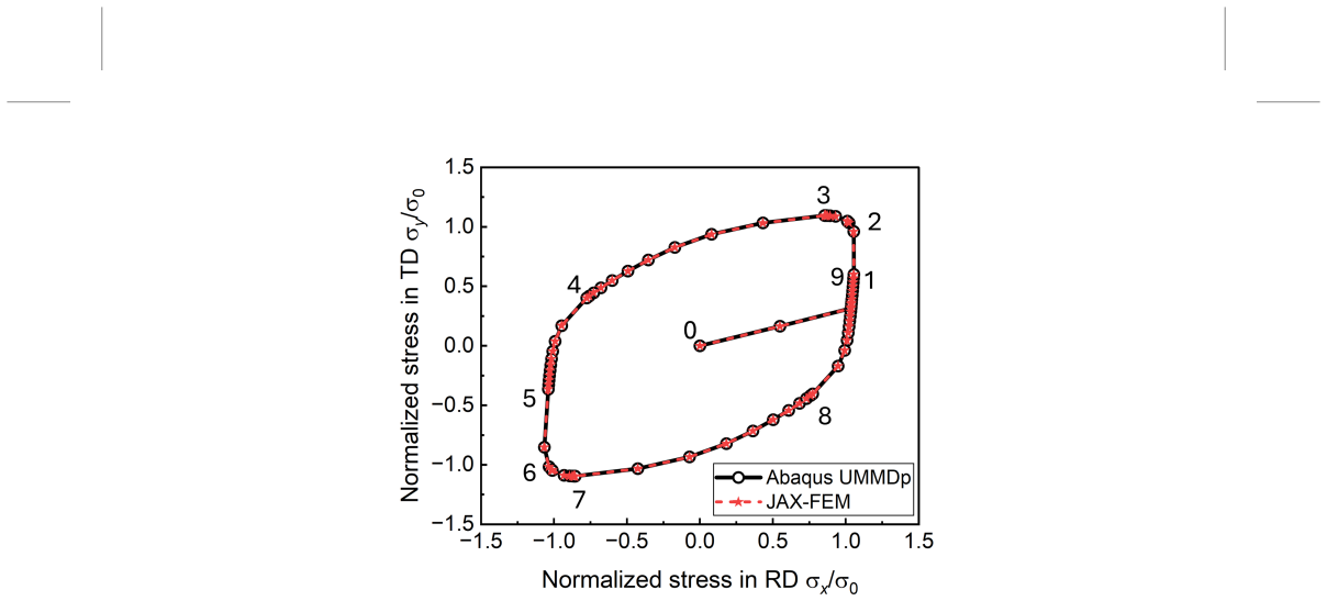
Summary. The manuscript presents JAX-FEM-ANISO, a fully differentiable GPU-accelerated finite-element framework built on JAX-FEM for forward simulation and inverse identification of finite-strain anisotropic plasticity (Hill–48 and Barlat Yld2004-18p). It implements Miehe’s modular logarithmic-strain formulation with F-bar kinematics, AD-derived consistent tangents and custom JVPs for local return mapping and spectral maps, GPU-resident residual/stiffness evaluation, sparse assembly, and linear solves (AMGX/CuDSS), plus discrete adjoint gradients for FEMU. Forward results are verified against Abaqus (flange drawing; single-element Barlat path). On ~3M DOF, a single H100 yields up to 9.4× wall-clock speedup versus a 24-core Abaqus CPU baseline. Adjoint gradients match central finite differences to <0.2% at h=10⁻⁶. Inverse studies on synthetic full-field displacements recover anisotropic yield/hardening parameters for information-rich tensile and cruciform specimens (with noise), two-region spatial heterogeneity, and a high-dimensional Barlat parameter set from a topology-optimized specimen.
Significance. If the reported accuracy and performance hold, this is a substantial systems and methods contribution for computational solid mechanics and Material Testing 2.0: it removes manual consistent-tangent derivation for advanced anisotropic models, makes high-dimensional FEMU gradients practical via reverse-mode AD, and demonstrates GPU scaling on million-DOF nonlinear problems. Strengths include careful Abaqus verification, explicit FD–AD gradient checks with the expected step-size U-curve, transparent reporting of Voce (Q,b) non-uniqueness while matching hardening curves, and progressive inverse demos up to Barlat Yld2004-18p and multi-material fields. These establish differentiable GPU FEM as a credible engine for simulation and synthetic-data inverse design; real DIC transfer remains future work as stated in §4.
major comments (2)
- Abstract and §4 claim a “practical high-throughput engine for … characterization” and that information-rich single tests can replace many conventional experiments. All inverse results (§3.3–3.6) use same-model synthetic displacements (optional i.i.d. Gaussian noise), not real DIC with imperfect BCs, incomplete observations, or model discrepancy—explicitly deferred to future work in §4. The algorithmic claims (AD gradients, GPU speedups, synthetic recovery) are supported; the characterization-engine phrasing overreaches the evidence. Please qualify abstract/conclusions/keywords so “single-test characterization” is framed as demonstrated on synthetic full-field data and as a pathway toward DIC-based MT2.0, not as an established experimental replacement.
- §3.5 titles and abstract language refer to “spatially varying material properties,” but the demonstration is two discrete material regions with piecewise-constant parameters (12 scalars), not a continuous field (e.g., nodal or element-wise parameter map). That is still a useful multi-material test and shows AD scaling with parameter count, but it does not yet establish continuous spatial-field identification. Clarify the claim (two-region heterogeneity vs. field reconstruction) and, if continuous fields are intended as a contribution, either add a small field example or soften the wording.
minor comments (6)
- Typos/grammar: “largly unexplored” (Introduction); “memeory demands,” “stiffness materix,” “uisng JAX” (§2.1); “V oce” spacing throughout (should be Voce); “non-finite solutions” is fine but check consistency of “finite-difference” hyphenation.
- Table 4: Abaqus 24-core reference is on Windows 11 while other Abaqus runs are on RHEL; note this more prominently when interpreting the 9.4× figure so readers do not over-interpret cross-platform wall-clock ratios.
- §3.2 gradient check: direction vector Di=0.1 is somewhat arbitrary; a brief note that relative component-wise errors (Table 6) are the primary verification is enough.
- §3.6 Barlat inverse: recovered coefficients differ from ground truth while yield surfaces match—good—but state explicitly in the table caption that coefficient non-uniqueness is expected and that surface/hardening agreement is the success metric.
- Figures 5, 14, 18, 26: ensure colorbars and deformed-mesh scales are readable in print; some multi-panel layouts are dense.
- Related work: briefly position against other differentiable FEM/plasticity efforts beyond JAX-FEM/JAX-CPFEM (e.g., other AD-enabled continuum codes) so novelty of the anisotropic finite-strain + inverse stack is sharper.
Circularity Check
No load-bearing circularity; inverse recoveries are standard same-model synthetic verification, gradients cross-checked by independent FD, and JAX-FEM base is an engineering substrate not a uniqueness claim.
-
self citation load bearing
[Abstract / §1 / §2.2.5 (JAX-FEM base)]
"Built on JAX-FEM, the framework exploits modern accelerator architectures by parallelizing the three major computational bottlenecks in nonlinear FEM... JAX-FEM provides a general-purpose, GPU-accelerated differentiable finite element framework..."
The implementation re-uses the authors’ own prior JAX-FEM library for elemental residual/stiffness kernels, sparse assembly and linear solves. This is ordinary engineering reuse of a software substrate rather than a load-bearing uniqueness or ansatz claim; the anisotropic constitutive update, custom JVPs, adjoint formulation and inverse results are independently derived and externally verified against Abaqus and finite differences. Flagged only as a minor self-citation that does not force any scientific conclusion.
full rationale
The paper implements Miehe’s modular logarithmic-strain finite-strain plasticity (Hill–48 and Yld2004-18p) inside an existing differentiable GPU FEM library, supplies consistent tangents and adjoints via custom JVPs and reverse-mode AD, and verifies forward solutions against Abaqus and objective gradients against central finite differences (absolute differences <0.2 % at h=10^{-6}). Inverse examples recover the very parameters used to generate the synthetic full-field displacements (with optional additive Gaussian noise); this is ordinary method verification, not a derivation that forces the result by construction, and the paper itself reports the well-known non-uniqueness of the (Q,b) hardening pair. The sole minor self-reference is the reuse of the authors’ prior JAX-FEM infrastructure for residual/stiffness evaluation and assembly; that infrastructure is an engineering substrate, not a uniqueness theorem or ansatz that closes the logical loop. Real DIC transfer is explicitly left to future work. Consequently the derivation chain is self-contained against external benchmarks and exhibits no circular reduction of the kind enumerated in the analyzer rules.
Assumptions & free parameters
free parameters (4)
- Constitutive parameter vector θ (Hill r_ij, Voce σ0/Q/b, Barlat c′/c′′ coefficients, m)
- Finite-difference step size h and AD regularization δ for spectral map
- L-BFGS-B convergence tolerances, parameter normalization bounds, noise scale δ_noise
- Adaptive time-step bounds (Δt_initial, Δt_min, Δt_max) and line-search β, η
assumptions (5)
- domain assumption Finite-strain anisotropic plasticity is adequately represented by Miehe’s additive logarithmic-strain modular framework with associative flow and isotropic Voce hardening.
- domain assumption Quasi-static equilibrium without body forces/inertia; F-bar kinematics control volumetric locking.
- standard math Discrete adjoint / reverse-mode AD through the time-discrete residual yields correct dJ/dθ for path-dependent plasticity when custom VJPs use the implicit-function theorem at local and global Newton levels.
- ad hoc to paper Synthetic full-field displacements (optionally with i.i.d. Gaussian noise) are a sufficient proxy to demonstrate inverse identification performance relevant to DIC-based Material Testing 2.0.
- domain assumption Automatic differentiation through spectral logarithmic strain can be made well-defined via small diagonal regularization or analytic Seth–Hill JVPs.
Cite this review
Pith. "Pith review of JAX-FEM-ANISO: Differentiable GPU-Accelerated Finite Element Framework for Inverse Identification of Finite-Strain Anisotropic Plasticity." pith.science (2026). https://pith.science/paper/7NJ7BEAY
@misc{pith2026260617390,
  author       = {Pith},
  title        = {Pith review of: JAX-FEM-ANISO: Differentiable GPU-Accelerated Finite Element Framework for Inverse Identification of Finite-Strain Anisotropic Plasticity},
  year         = {2026},
  howpublished = {\url{https://pith.science/paper/7NJ7BEAY}},
  note         = {Machine review of arXiv:2606.17390}
}
abstract
We present a fully differentiable, GPU-accelerated finite element framework JAX-FEM-ANISO, for forward simulation and inverse parameter identification of finite-strain anisotropic plasticity. Built on JAX-FEM, the framework exploits modern accelerator architectures by parallelizing the three major computational bottlenecks in nonlinear FEM: elemental weak-form and tangent-stiffness evaluation, global sparse matrix assembly, and sparse linear solution. For a large-scale forward problem with 3 million degrees of freedom, JAX-FEM-ANISO on a single NVIDIA H100 GPU achieves up to 9.4$\times$ speed-up over a 24-core CPU Abaqus baseline. Automatic differentiation is applied through the constitutive update and solver workflow, providing consistent Jacobians for complex constitutive models without manual derivation and accurate gradients for PDE-constrained inverse analysis. Compared with finite differences, the JAX-AD gradients avoid step-size sensitivity and provide the required sensitivities at substantially lower computational cost. For inverse characterization, we combine information-rich, topology-optimized heterogeneous specimens with full-field displacement data to identify advanced constitutive model parameters from a single test, replacing what would otherwise require many conventional experiments. We demonstrate accurate recovery of anisotropic yield and hardening parameters in progressively challenging settings, including uniform and spatially varying material properties. The resulting AD-based formulation enables efficient optimization in high-dimensional parameter spaces where finite-difference approaches are computationally infeasible. These results establish differentiable, GPU-accelerated FEM as a practical high-throughput engine for simulation, characterization, and optimization workflows in advanced manufacturing.
Figures


Figures from the paper (25 more)




Reference graph
Works this paper leans on
-
[1]
J. C. Simo and T. J. R. Hughes.Computational Inelasticity. Springer, New York, NY , 1998
1998
-
[2]
Belytschko, W
T. Belytschko, W. K. Liu, and B. Moran.Nonlinear Finite Elements for Continua and Structures. John Wiley & Sons, Chichester, UK, 2000
2000
-
[3]
R. Hill. A theory of the yielding and plastic flow of anisotropic metals.Proceedings of the Royal Society of London. Series A. Mathematical and Physical Sciences, 193(1033):281–297, 1948
1948
-
[4]
Barlat, J
F. Barlat, J. C. Brem, J. W. Yoon, K. Chung, R. E. Dick, D. J. Lege, F. Pourboghrat, S.-H. Choi, and E. Chu. Plane stress yield function for aluminum alloy sheets—part 1: theory.International Journal of Plasticity, 19(9):1297–1319, 2003
2003
-
[5]
Barlat, H
F. Barlat, H. Aretz, J. W. Yoon, M. E. Karabin, J. C. Brem, and R. E. Dick. Linear transformation-based anisotropic yield functions.International Journal of Plasticity, 21(5):1009–1039, 2005
2005
-
[6]
E. A. de Souza Neto, D. Peri´c, and D. R. J. Owen.Computational Methods for Plasticity: Theory and Applications. John Wiley & Sons, Chichester, UK, 2008
2008
-
[7]
Michaleris, D
P. Michaleris, D. A. Tortorelli, and C. A. Vidal. Tangent operators and design sensitivity formulations for transient non- linear coupled problems with applications to elastoplasticity.International Journal for Numerical Methods in Engineering, 37(14):2471–2499, 1994
1994
-
[8]
Miehe, N
C. Miehe, N. Apel, and M. Lambrecht. Anisotropic additive plasticity in the logarithmic strain space: modular kinematic formulation and implementation based on incremental minimization principles for standard materials.Computer Methods in Applied Mechanics and Engineering, 191:5383–5425, 2002
2002
Show all 68 references
-
[9]
N. Aravas. On the numerical integration of a class of pressure-dependent plasticity models.International Journal for Numerical Methods in Engineering, 24(7):1395–1416, 1987
1987
-
[10]
Güner, C
A. Güner, C. Soyarslan, A. Brosius, and A. E. Tekkaya. Characterization of anisotropy of sheet metals employing inhomogeneous strain fields for Yld2000-2D yield function.International Journal of Solids and Structures, 49(25):3517– 3527, 2012
2012
-
[11]
J. H. Kim, F. Barlat, F. Pierron, and M. G. Lee. Determination of anisotropic plastic constitutive parameters using the virtual fields method.Experimental Mechanics, 54(7):1189–1204, 2014
2014
-
[12]
M. A. Sutton, J.-J. Orteu, and H. Schreier.Image Correlation for Shape, Motion and Deformation Measurements: Basic Concepts, Theory and Applications. Springer, New York, NY , 2009
2009
-
[13]
Bertin, F
M. Bertin, F. Hild, and S. Roux. On the identifiability of Hill-1948 plasticity model with a single biaxial test on very thin sheet.Strain, 53(5):e12233, 2017
1948
-
[14]
Coppieters, T
S. Coppieters, T. Hakoyama, D. Debruyne, S. Takahashi, and T. Kuwabara. Inverse yield locus identification of sheet metal using a complex cruciform in biaxial tension and digital image correlation.Proceedings, 60(2):382, 2018
2018
-
[15]
Zhang, M
Y . Zhang, M. Rossi, R. Pettermann, and C. Sommitsch. Inverse identification of plastic anisotropy through multiple non-conventional mechanical experiments.International Journal of Solids and Structures, 285:112534, 2023
2023
-
[16]
Pierron and M
F. Pierron and M. Grédiac. Towards material testing 2.0. a review of test design for identification of constitutive parameters from full-field measurements.Strain, 57(1):e12370, 2021
2021
-
[17]
J. M. P. Martins, A. Andrade-Campos, and S. Thuillier. Comparison of inverse identification strategies for constitutive mechanical models using full-field measurements.International Journal of Mechanical Sciences, 145:330–345, 2018
2018
-
[18]
Marek, F
A. Marek, F. M. Davis, M. Rossi, and F. Pierron. Extension of the sensitivity-based virtual fields to large deformation anisotropic plasticity.International Journal of Material Forming, 12(3):457–476, 2019
2019
-
[19]
Zhang, M
Y . Zhang, M. Rossi, J. Reisch, R. Pettermann, and C. Sommitsch. Enhancing the information-richness of sheet metal specimens for inverse identification of plastic anisotropy through strain fields.International Journal of Mechanical Sciences, 214:106891, 2022
2022
-
[20]
Conde, Y
M. Conde, Y . Zhang, J. Henriques, S. Coppieters, and A. Andrade-Campos. Design and validation of a heterogeneous interior notched specimen for inverse material parameter identification.Finite Elements in Analysis and Design, 214:103866, 2023
2023
-
[21]
Gonçalves, S
M. Gonçalves, S. Thuillier, and A. Andrade-Campos. Inverse identification of anisotropic plasticity model parameters using FEMU and a heterogeneous test. InESAFORM 2025, volume 54, pages 1548–1557, 2025
2025
-
[22]
D. T. Seidl and B. N. Granzow. Calibration of elastoplastic constitutive model parameters from full-field data with automatic differentiation-based sensitivities.International Journal for Numerical Methods in Engineering, 123(1):69–100, 2022
2022
-
[23]
Kumar, D
S. Kumar, D. T. Seidl, B. N. Granzow, J. Yang, and J. N. Fuhg. A comparative study of calibration techniques for finite strain elastoplasticity: Numerically-exact sensitivities for FEMU and VFM.Computer Methods in Applied Mechanics and Engineering, 444:118159, 2025
2025
-
[24]
C. C. Margossian. A review of automatic differentiation and its efficient implementation.Wiley Interdisciplinary Reviews: Data Mining and Knowledge Discovery, 9(4):e1305, 2019
2019
-
[25]
Rothe and S
S. Rothe and S. Hartmann. Automatic differentiation for stress and consistent tangent computation.Archive of Applied Mechanics, 85(8):1103–1125, 2015
2015
-
[26]
Dummer, M
A. Dummer, M. Neuner, P. Gamnitzer, and G. Hofstetter. Robust and efficient implementation of finite strain generalized continuum models for material failure: Analytical, numerical, and automatic differentiation with hyper-dual numbers. Computer Methods in Applied Mechanics an...
2024
-
[27]
Y . Jia, W. Li, and X. S. Zhang. Multimaterial topology optimization of elastoplastic composite structures.Journal of the Mechanics and Physics of Solids, 196:106018, 2025
2025
-
[28]
Jia and X
Y . Jia and X. S. Zhang. Multimaterial topology optimization for finite strain elastoplasticity: theory, methods, and applications. Computer Methods in Applied Mechanics and Engineering, 449:118445, 2026
2026
-
[29]
Bradbury, R
J. Bradbury, R. Frostig, P. Hawkins, M. J. Johnson, C. Leary, D. Maclaurin, G. Necula, A. Paszke, J. Vander- Plas, S. Wanderman-Milne, and Q. Zhang. JAX: composable transformations of Python+NumPy programs. http: //github.com/google/jax, 2018
2018
-
[30]
Paszke, S
A. Paszke, S. Gross, F. Massa, A. Lerer, J. Bradbury, G. Chanan, et al. PyTorch: An imperative style, high-performance deep learning library.Advances in Neural Information Processing Systems, 32, 2019
2019
-
[31]
M. Macklin. Warp: A high-performance python framework for GPU simulation and graphics. InNVIDIA GPU Technology Conference (GTC), volume 3, 2022
2022
-
[32]
NVIDIA H100 Tensor Core GPU datasheet
NVIDIA Corporation. NVIDIA H100 Tensor Core GPU datasheet. https://resources.nvidia.com/ en-us-hopper-architecture/nvidia-tensor-core-gpu-datasheet, 2023
2023
-
[33]
Intel Xeon 6952P Processor specifications
Intel Corporation. Intel Xeon 6952P Processor specifications. https://www.intel.com/content/www/us/en/ products/sku/241643/intel-xeon-6952p-processor-480m-cache-2-10-ghz/specifications.html, 2026
2026
-
[34]
Williams, A
S. Williams, A. Waterman, and D. Patterson. Roofline: an insightful visual performance model for multicore architectures. Communications of the ACM, 52(4):65–76, 2009
2009
-
[35]
Martínez-Frutos, P
J. Martínez-Frutos, P. J. Martínez-Castejón, and D. Herrero-Pérez. Fine-grained GPU implementation of assembly-free iterative solver for finite element problems.Computers&Structures, 157:9–18, 2015
2015
-
[36]
Aissa, T
M. Aissa, T. Verstraete, and C. Vuik. Toward a GPU-aware comparison of explicit and implicit CFD simulations on structured meshes.Computers&Mathematics with Applications, 74(1):201–217, 2017
2017
-
[37]
Stavroulakis, D
G. Stavroulakis, D. G. Giovanis, V . Papadopoulos, and M. Papadrakakis. A GPU domain decomposition solution for spectral stochastic finite element method.Computer Methods in Applied Mechanics and Engineering, 327:392–410, 2017
2017
-
[38]
Ghysels and R
P. Ghysels and R. Synk. High performance sparse multifrontal solvers on modern GPUs.Parallel Computing, 110:102897, 2022
2022
-
[39]
F. Li, F. Zou, and J. Rao. A multi-GPU and CUDA-aware MPI-based spectral element formulation for ultrasonic wave propagation in solid media.Ultrasonics, 134:107049, 2023
2023
-
[40]
Kiran, D
U. Kiran, D. Sharma, and S. S. Gautam. Development of GPU-based matrix-free strategies for large-scale elastoplasticity analysis using conjugate gradient solver.International Journal for Numerical Methods in Engineering, 125(7):e7421, 2024
2024
-
[41]
S. Hong, G. Jang, and W. K. Jeong. MG-FIM: A multi-GPU fast iterative method using adaptive domain decomposition. SIAM Journal on Scientific Computing, 44(1):C54–C76, 2022
2022
-
[42]
S. Liao, A. Golgoon, M. Mozaffar, and J. Cao. Efficient GPU-accelerated thermomechanical solver for residual stress prediction in additive manufacturing.Computational Mechanics, 71(5):879–893, 2023
2023
-
[43]
E. A. Träff, A. Rydahl, S. Karlsson, O. Sigmund, and N. Aage. Simple and efficient GPU accelerated topology optimisation: Codes and applications.Computer Methods in Applied Mechanics and Engineering, 410:116043, 2023
2023
-
[44]
Kiran, D
U. Kiran, D. Sharma, and S. S. Gautam. An efficient framework for matrix-free SpMV computation on GPU for elastoplastic problems.Mathematics and Computers in Simulation, 216:318–346, 2024
2024
-
[45]
Karatarakis, P
A. Karatarakis, P. Karakitsios, and M. Papadrakakis. GPU accelerated computation of the isogeometric analysis stiffness matrix.Computer Methods in Applied Mechanics and Engineering, 269:334–355, 2014
2014
-
[46]
T. Xue, S. Liao, Z. Gan, C. Park, X. Xie, W. K. Liu, and J. Cao. JAX-FEM: A differentiable GPU-accelerated 3d finite element solver for automatic inverse design and mechanistic data science.Computer Physics Communications, 291:108802, 2023
2023
-
[47]
F. Hu, S. Niezgoda, T. Xue, and J. Cao. Efficient GPU-computing simulation platform JAX-CPFEM for differentiable crystal plasticity finite element method.npj Computational Materials, 11(1):46, 2025
2025
-
[48]
F. Hu, R. Zhou, K. Ryou, R. Zha, S. Niezgoda, T. Xue, and J. Cao. An efficient graphical processing unit-accelerated calibration of crystal plasticity model parameters by multi-objective optimization with automatic differentiation-based sensitivities.Journal of Applied Mechani...
2026
-
[49]
B. P. Ferreira and M. A. Bessa. Automatically differentiable model updating (ADiMU): conventional, hybrid, and neural network material model discovery including history-dependency.arXiv preprint arXiv:2505.07801, 2025
2025 arXiv
-
[50]
Knapik, S
S. Knapik, S. Deng, L. Wang, A. Chandrasekhar, W. K. Liu, J. Cao, and W. Chen. Co-design of geometry and thermal-elastic gradient alloy distribution with temperature-dependent material properties.Structural and Multidisciplinary Optimization, 68(7):127, 2025
2025
-
[51]
J. P. Leonor and G. J. Wagner. GO-MELT: GPU-optimized multilevel execution of LPBF thermal simulations.Computer Methods in Applied Mechanics and Engineering, 426:116977, 2024
2024
-
[52]
AmgX: GPU accelerated linear solvers.https://developer.nvidia.com/amgx, 2026
NVIDIA Corporation. AmgX: GPU accelerated linear solvers.https://developer.nvidia.com/amgx, 2026
2026
-
[53]
E. A. de Souza Neto, D. Peric, and D. R. Owen.Computational Methods for Plasticity: Theory and Applications. John Wiley & Sons, Chichester, UK, 2011
2011
-
[54]
W. M. Scherzinger. A return mapping algorithm for isotropic and anisotropic plasticity models using a line search method. Computer Methods in Applied Mechanics and Engineering, 317:526–553, 2017
2017
-
[55]
Scalet and F
G. Scalet and F. Auricchio. Computational methods for elastoplasticity: An overview of conventional and less-conventional approaches.Archives of Computational Methods in Engineering, 25(3):545–589, 2018
2018
-
[56]
Alfano, L
G. Alfano, L. Rosati, and N. Valoroso. A tangent–secant approach to rate-independent elastoplasticity: formulations and computational issues.Computer Methods in Applied Mechanics and Engineering, 179(3–4):379–405, 1999
1999
-
[57]
Miehe and M
C. Miehe and M. Lambrecht. Algorithms for computation of stresses and elasticity moduli in terms of Seth–Hill’s family of generalized strain tensors.Communications in Numerical Methods in Engineering, 17(5):337–353, 2001
2001
-
[58]
Z. Fu, T. J. Lewis, R. M. Kirby, and R. T. Whitaker. Architecting the finite element method pipeline for the GPU.Journal of Computational and Applied Mathematics, 257:195–211, 2014
2014
-
[59]
Meng, B.-L
H.-T. Meng, B.-L. Nie, S. Wong, C. Macon, and J.-M. Jin. GPU accelerated finite-element computation for electromagnetic analysis.IEEE Antennas and Propagation Magazine, 56(2), 2014
2014
-
[60]
Kiran, D
U. Kiran, D. Sharma, and S. S. Gautam. GPU-warp based finite element matrices generation and assembly using coloring method.Journal of Computational Design and Engineering, 6(5):705–718, 2019
2019
-
[61]
M. B. Giles and N. A. Pierce. An introduction to the adjoint approach to design.Flow, Turbulence and Combustion, 65:393–415, 2000
2000
-
[62]
Xu and E
K. Xu and E. Darve. Physics constrained learning for data-driven inverse modeling from sparse observations.Journal of Computational Physics, 453:110938, 2022
2022
-
[63]
Papadopoulos and J
P. Papadopoulos and J. Lu. A general framework for the numerical solution of problems in finite elasto-plasticity.Computer Methods in Applied Mechanics and Engineering, 159(1–2):1–18, 1998
1998
-
[64]
unified material model driver for plasticity (UMMDp)
H. Takizawa, K. Oide, K. Suzuki, T. Yamanashi, T. Inoue, T. Ida, T. Nagai, and T. Kuwabara. Development of the user subroutine library “unified material model driver for plasticity (UMMDp)” for various anisotropic yield functions.Journal of Physics: Conference Series, 1063:012...
2018
-
[65]
Tammas-Williams and I
S. Tammas-Williams and I. Todd. Design for additive manufacturing with site-specific properties in metals and alloys. Scripta Materialia, 135:105–110, 2017
2017
-
[66]
Gonçalves, A
M. Gonçalves, A. Andrade-Campos, and B. Barroqueiro. On the design of mechanical heterogeneous specimens using multilevel topology optimization.Advances in Engineering Software, 175:103314, 2023
2023
-
[67]
Gonçalves, M
M. Gonçalves, M. G. Oliveira, S. Thuillier, and A. Andrade-Campos. Key performance indicators for heterogeneous mechanical tests.International Journal of Mechanical Sciences, 264:108821, 2024
2024
-
[68]
Efficient and modular implicit differentiation.Advances in neural information processing systems, 35:5230–5242, 2022
Mathieu Blondel, Quentin Berthet, Marco Cuturi, Roy Frostig, Stephan Hoyer, Felipe Llinares-López, Fabian Pedregosa, and Jean-Philippe Vert. Efficient and modular implicit differentiation.Advances in neural information processing systems, 35:5230–5242, 2022
2022
Reviewed July 14, 2026 · model on record in the stance chip above.
Discussion (0). Continue with ORCID to comment.