Edge Flow: A Tractable and Predictive Continuous-Time Model for Gradient Descent at the Edge of Stability
Pith reviewed 2026-06-27 01:14 UTC · model grok-4.3
The pith
Gradient descent at the edge of stability follows three coupled ODEs whose feedback loop automatically stabilizes sharpness near 2/η.
A machine-rendered reading of the paper's core claim, the machinery that carries it, and where it could break.
Core claim
Edge Flow is a system of three coupled ordinary differential equations that models gradient descent at the edge of stability. The center follows a modified gradient flow on a symmetrized loss. The direction evolves by Rayleigh quotient dynamics that track a top eigenvector of the Hessian. The magnitude grows or decays exponentially depending on whether sharpness exceeds or falls below 2/η. Sharpness stabilization emerges automatically from the coupled dynamics via a self-stabilization feedback loop. The resulting continuous-time model admits a discretization that requires only two gradient evaluations and one Hessian-vector product per iteration.
What carries the argument
Edge Flow, the system of three coupled ODEs that decomposes dynamics into a center (modified gradient flow on symmetrized loss), a direction (Rayleigh quotient dynamics), and a magnitude (exponential growth or decay set by sharpness relative to 2/η).
If this is right
- Discretizing Edge Flow requires only two gradient evaluations and one Hessian-vector product at each iteration.
- The model tracks gradient descent trajectories at least as faithfully as earlier continuous-time EoS models while also resolving the oscillation of sharpness at the onset of the regime.
- The coupled dynamics supply a principled framework for understanding when instabilities arise and for designing interventions that mitigate them.
Where Pith is reading between the lines
- The same decomposition could be tested on optimization algorithms other than plain gradient descent to check whether self-stabilization is a broader discrete phenomenon.
- The explicit ODE system offers a low-cost simulation testbed for exploring learning-rate schedules or regularizers before full-scale training runs.
- If the self-stabilization loop proves robust, it may suggest new ways to choose step sizes that deliberately ride the edge rather than avoid it.
Load-bearing premise
The dynamics of gradient descent at EoS can be faithfully decomposed into a center obeying modified gradient flow on a symmetrized loss, a direction evolving by Rayleigh quotient dynamics, and an oscillation magnitude that grows or decays exponentially according to whether sharpness exceeds 2/η, with the three components coupled so that self-stabilization arises automatically.
What would settle it
Integrate Edge Flow alongside actual gradient descent on a network known to enter the edge-of-stability regime and observe that the predicted parameter trajectories or sharpness time series diverge substantially from the recorded run.
Figures


read the original abstract
Gradient descent in deep learning may operate at the edge of stability (EoS), a regime in which the largest eigenvalue of the loss Hessian hovers near the stability threshold $2/\eta$, where $\eta$ is the learning rate. Classical analysis tools such as gradient flow and the descent lemma do not apply here, motivating the search for a continuous-time model valid at EoS. We propose Edge Flow, a system of three coupled ordinary differential equations that provides a tractable, faithful, and predictive model of gradient descent dynamics at EoS. Edge Flow decomposes the dynamics into a center, an oscillation direction, and an oscillation magnitude. The center follows a modified gradient flow on a symmetrized loss; the direction tracks a top eigenvector of the Hessian via Rayleigh quotient dynamics; and the magnitude grows or decays exponentially depending on whether the sharpness exceeds or falls below the threshold $2/\eta$. Crucially, sharpness stabilization emerges from the coupled dynamics via a self-stabilization feedback loop. Discretizing Edge Flow only requires two gradient evaluations and one Hessian--vector product at each iteration. We demonstrate empirically that Edge Flow tracks the dynamics of gradient descent at least as faithfully as previously proposed continuous-time EoS models, while in addition resolving the oscillation of the sharpness at the onset of EoS, and that it provides a principled framework for understanding and mitigating instabilities in this regime.
Editorial analysis
A structured set of objections, weighed in public.
Referee Report
Summary. The paper proposes Edge Flow, a system of three coupled ODEs modeling gradient descent at the edge of stability (EoS). It decomposes the dynamics into a center following modified gradient flow on a symmetrized loss, a direction evolving via Rayleigh quotient dynamics to track the top Hessian eigenvector, and an oscillation magnitude that grows or decays exponentially according to whether sharpness exceeds or falls below 2/η. The central claim is that sharpness stabilization emerges automatically from the coupling via a self-stabilization feedback loop. Discretization requires two gradient evaluations and one Hessian-vector product per iteration. Empirical results are said to show that Edge Flow tracks GD at least as faithfully as prior continuous-time EoS models while additionally resolving sharpness oscillations at EoS onset and providing a framework for instabilities.
Significance. If the derivations establish that stabilization is a derived consequence of the coupling (rather than presupposed by the functional forms) and if the empirical comparisons include rigorous quantitative metrics with error analysis, the model could supply a tractable continuous-time tool for analyzing a regime where classical gradient flow and descent lemma do not apply. The explicit, low-cost discretization (two gradients + one HVP) is a concrete strength that could enable practical use. The work addresses a practically relevant phenomenon in deep learning training.
major comments (2)
- [Abstract] Abstract: the claim that 'sharpness stabilization emerges from the coupled dynamics via a self-stabilization feedback loop' is load-bearing for the contribution, yet the abstract supplies no derivation steps, explicit equations for the three ODEs, or analysis showing that the stabilization is a consequence of the coupling rather than built into the chosen functional forms for center, direction, and magnitude. This must be shown explicitly (e.g., via the ODE definitions and any subsequent analysis section) to substantiate the central claim.
- [Abstract] Abstract: the assertions that the model is 'faithful and predictive' and 'tracks the dynamics of gradient descent at least as faithfully as previously proposed continuous-time EoS models' rest on unspecified experiments with no reported quantitative metrics, error bounds, or comparison tables. Without these, the faithfulness claim cannot be evaluated and is central to the paper's empirical contribution.
minor comments (1)
- [Abstract] The discretization cost is stated clearly, but the abstract would benefit from a brief parenthetical note on how the two gradients and one HVP arise from the ODE discretization.
Simulated Author's Rebuttal
We thank the referee for their constructive comments, which highlight opportunities to strengthen the presentation of our central claims. We address each major comment below with references to the full manuscript and indicate planned revisions.
read point-by-point responses
-
Referee: [Abstract] Abstract: the claim that 'sharpness stabilization emerges from the coupled dynamics via a self-stabilization feedback loop' is load-bearing for the contribution, yet the abstract supplies no derivation steps, explicit equations for the three ODEs, or analysis showing that the stabilization is a consequence of the coupling rather than built into the chosen functional forms for center, direction, and magnitude. This must be shown explicitly (e.g., via the ODE definitions and any subsequent analysis section) to substantiate the central claim.
Authors: The full manuscript defines the three ODEs explicitly in Section 3 (center as modified gradient flow on the symmetrized loss, direction via Rayleigh quotient dynamics, and magnitude via exponential growth/decay conditioned on sharpness relative to 2/η). Section 4 then analyzes the coupled system and derives that the self-stabilization feedback loop arises from the interaction: the magnitude modulates the effective sharpness experienced by the center, which in turn influences the direction and feeds back to bound the magnitude, rather than the threshold behavior being independently imposed. We agree the abstract does not sufficiently signal this structure or the derivation and will revise it to include a concise reference to the ODE components and the emergence of stabilization from their coupling. revision: yes
-
Referee: [Abstract] Abstract: the assertions that the model is 'faithful and predictive' and 'tracks the dynamics of gradient descent at least as faithfully as previously proposed continuous-time EoS models' rest on unspecified experiments with no reported quantitative metrics, error bounds, or comparison tables. Without these, the faithfulness claim cannot be evaluated and is central to the paper's empirical contribution.
Authors: Section 5 presents the empirical evaluation, including direct trajectory comparisons against GD and prior EoS models (e.g., via integrated squared error on parameter paths and sharpness time series), with reported error norms, oscillation amplitude statistics, and qualitative resolution of sharpness oscillations at EoS onset. While these metrics appear in the main text and appendix, the abstract does not reference them. We will revise the abstract to briefly note the use of quantitative trajectory and sharpness metrics in the comparisons, and we will ensure a summary comparison table is clearly highlighted in the main body. revision: partial
Circularity Check
No significant circularity; model construction is self-contained
full rationale
The provided abstract and reader summary describe a proposed three-component ODE system (center on symmetrized loss, Rayleigh-quotient direction, exponential magnitude) whose coupling is asserted to produce self-stabilization of sharpness. No equations, self-citations, fitted parameters renamed as predictions, or ansatzes smuggled via prior work are visible in the text. The discretization cost is stated explicitly and parameter-free. Because no load-bearing step reduces by construction to its own inputs or to a self-citation chain, the derivation chain does not exhibit circularity. The central claim remains an independent modeling proposal whose faithfulness is to be checked against external GD trajectories rather than by internal redefinition.
Axiom & Free-Parameter Ledger
axioms (2)
- ad hoc to paper Gradient descent at EoS can be decomposed into center, oscillation direction, and oscillation magnitude components whose coupling produces self-stabilization.
- ad hoc to paper The center follows a modified gradient flow on a symmetrized loss.
invented entities (1)
-
Edge Flow (three coupled ODEs with center, direction, and magnitude)
no independent evidence
Reference graph
Works this paper leans on
-
[1]
A. Lewkowycz, Y. Bahri, E. Dyer, J. Sohl-Dickstein, and G. Gur-Ari. The large learning rate phase of deep learning: the catapult mechanism.arXiv preprint arXiv:2003.02218,
arXiv 2003
-
[2]
P. Marion and Y.-H. Wu. Understanding diffusion models requires rethinking (again) generaliza- tion.arXiv preprint arXiv:2605.06077,
-
[3]
Accessed: 2026-06-15. R. Mulayoff and T. Michaeli. Exact mean square linear stability analysis for SGD. InConference on Learning Theory (COLT), volume 247, pages 3915–3969,
2026
-
[4]
R. Mulayoff and S. U. Stich. On the stability of nonlinear dynamics in GD and SGD: Beyond quadratic potentials.arXiv preprint arXiv:2602.14789,
-
[5]
12 E. Regis and S. Chewi. Rod flow: A continuous-time model for gradient descent at the edge of stability.arXiv preprint arXiv:2602.01480,
-
[6]
Y.-H. Wu, P. Marion, G. Biau, and C. Boyer. Taking a big step: Large learning rates in denoising score matching prevent memorization. InConference on Learning Theory, volume 291, pages 5718–5756, 2025b. C. Xing, D. Arpit, C. Tsirigotis, and Y. Bengio. A walk with SGD.arXiv preprint arXiv:1802.08770,
-
[7]
and Rod Flow (Regis and Chewi, 2026). These two models as well as Edge Flow share the same starting point: at EoS, the GD trajectory splits into a slowly moving center and a fast oscillation, and one seeks autonomous dynamics for the slow variables. They differ in two essential choices. The first is how the oscillation isrepresented: a constraint on the s...
2026
-
[8]
Running Gradient Flow yields the same dynamics as Rod Flow
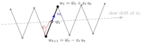
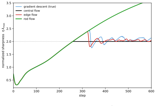
Central Flow pins the sharpness at2and Edge Flow tracks the gradient-descent oscillation around it, whereas Rod Flow does not stabilize the sharpness and drifts upward. Running Gradient Flow yields the same dynamics as Rod Flow. doing a Taylor expansion of the gradients, we obtain that the magnitude of the oscillations evolves according to d(x2 t ) dt ≈u ...
2026
-
[9]
The two settings share most of their setup, which we describe first
and for the rod-flow comparison (Figure 6). The two settings share most of their setup, which we describe first. Common setup.All experiments are implemented inPyTorch, building on the publicly available Central Flows codebase of Cohen et al. (2025) (https://github.com/locuslab/ central_flows), which we extend to implement Edge Gradient Descent (see pseud...
2025
-
[10]
Test metrics are evaluated on the CIFAR-10 test images of the same four classes, and the network-output panels display the model’s four output logits on a single fixed test example
combine three architectures with two losses—mean-squared error (MSE) regressed onto one-hot labels and softmax cross-entropy (CE)—and use n = 1000training examples (250per class), with4output units. Test metrics are evaluated on the CIFAR-10 test images of the same four classes, and the network-output panels display the model’s four output logits on a sin...
2025
-
[11]
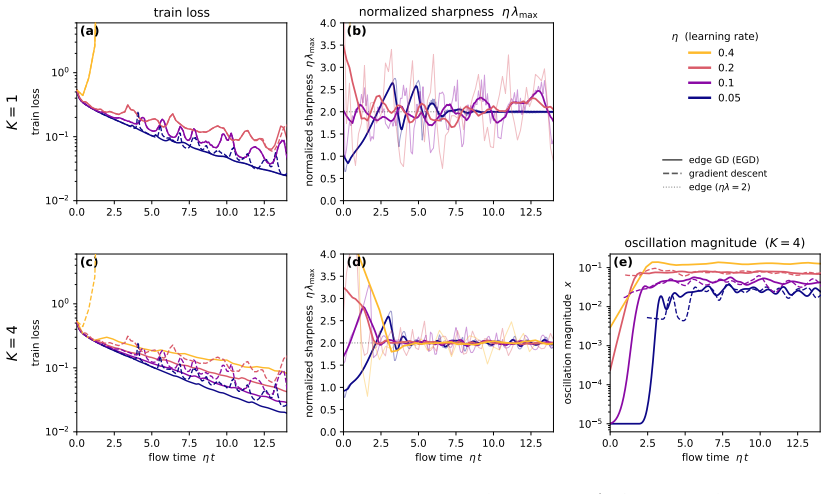
Refining the discretization of the center thus seems to extend the range of stable learning rates, as discussed in Section 4.3
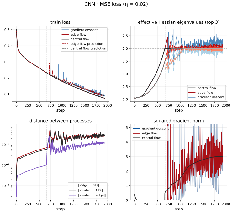
Pushing further, K = 4also eventually diverges, around η = 0.5. Refining the discretization of the center thus seems to extend the range of stable learning rates, as discussed in Section 4.3. 17 0 250 500 750 1000 1250 1500 1750 2000 step 0.1 0.2 0.3 0.4 0.5 train loss gradient descent edge flow central flow edge flow prediction central flow prediction 0 ...
2000
-
[12]
central flow edge flow gradient descent 0 250 500 750 1000 1250 1500 1750 2000 step 10 4 10 3 10 2 distance between processes edge GD central GD central edge 0 250 500 750 1000 1250 1500 1750 2000 step 0 1 2 3 4 5 squared gradient norm gradient descent edge flow central flow 600 800 1000 1200 1400 1600 1800 step 0.0000 0.0001 0.0002 0.0003 0.0004 0.0005 0...
2000
-
[13]
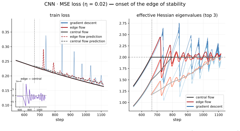
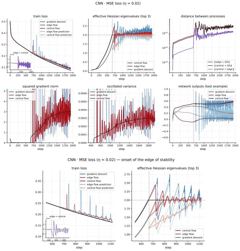
The inset on the train losses panels shows the small gap between the Edge Flow and Central Flow centers
central flow edge flow gradient descent 600 800 1000 5 0 5 1e 4 edge central CNN · MSE loss ( = 0.02) onset of the edge of stability Figure 7:CNN with MSE loss(η = 0.02): full set of metrics (top) and zoom on the onset of the edge of stability (bottom). The inset on the train losses panels shows the small gap between the Edge Flow and Central Flow centers...
2000
-
[14]
edge flow gradient descent 0 500 1000 1500 2000 2500 3000 step 10 5 10 4 10 3 10 2 10 1 distance between processes edge GD 0 500 1000 1500 2000 2500 3000 step 0 10 20 30 40 50 60 70 squared gradient norm gradient descent edge flow 1000 1250 1500 1750 2000 2250 2500 2750 step 0.0000 0.0002 0.0004 0.0006 0.0008 0.0010 0.0012 0.0014 oscillated variance gradi...
2000
-
[15]
Full set of metrics (top) and zoom on the onset of the edge of stability (bottom)
edge flow gradient descent CNN · cross-entropy loss ( = 0.01) onset of the edge of stability Figure 8:CNN with cross-entropy loss(η = 0.01). Full set of metrics (top) and zoom on the onset of the edge of stability (bottom). 19 0 500 1000 1500 2000 2500 3000 3500 step 0.1 0.2 0.3 0.4 0.5 train loss gradient descent edge flow edge flow prediction 0 500 1000...
2000
-
[16]
edge flow gradient descent 0 500 1000 1500 2000 2500 3000 3500 step 10 2 10 1 distance between processes edge GD 0 500 1000 1500 2000 2500 3000 3500 step 0.0 0.5 1.0 1.5 2.0 2.5 3.0 squared gradient norm gradient descent edge flow 0 500 1000 1500 2000 2500 3000 3500 step 0.00000 0.00005 0.00010 0.00015 0.00020 0.00025 0.00030 0.00035 oscillated variance g...
2000
-
[17]
Full set of metrics (top) and zoom on the onset of the edge of stability (bottom)
edge flow gradient descent ResNet · MSE loss ( = 0.02) onset of the edge of stability Figure 9:ResNet with MSE loss(η = 0.02). Full set of metrics (top) and zoom on the onset of the edge of stability (bottom). 20 0 500 1000 1500 2000 2500 3000 3500 step 0.0 0.2 0.4 0.6 0.8 1.0 1.2 1.4 train loss gradient descent edge flow edge flow prediction 0 500 1000 1...
2000
-
[18]
edge flow gradient descent 0 500 1000 1500 2000 2500 3000 3500 step 10 3 10 2 10 1 distance between processes edge GD 0 500 1000 1500 2000 2500 3000 3500 step 0.0 2.5 5.0 7.5 10.0 12.5 15.0 17.5 squared gradient norm gradient descent edge flow 0 500 1000 1500 2000 2500 3000 step 0.0000 0.0002 0.0004 0.0006 0.0008 0.0010 0.0012 oscillated variance gradient...
2000
-
[19]
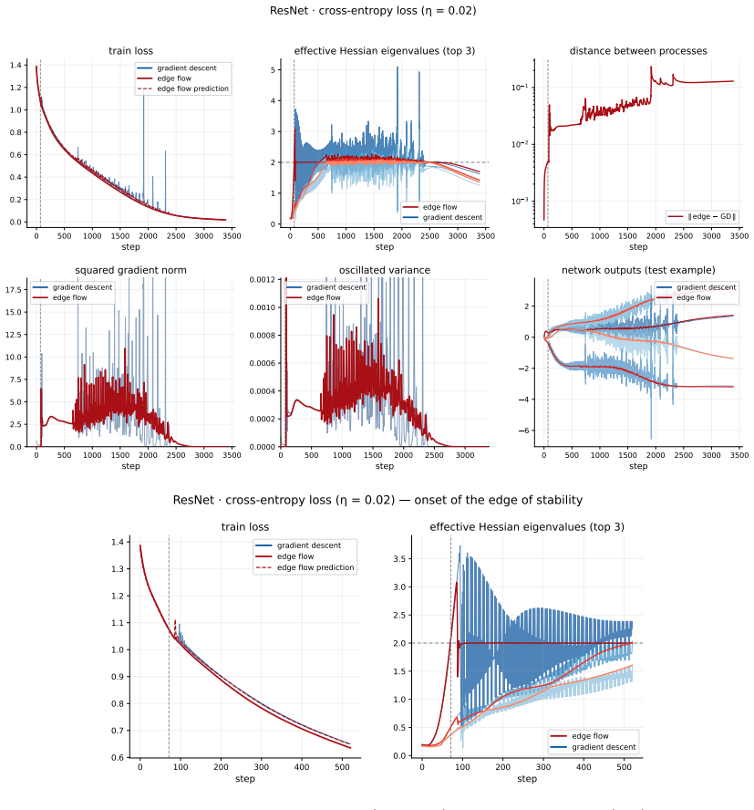
Full set of metrics (top) and zoom on the onset of the edge of stability (bottom)
edge flow gradient descent ResNet · cross-entropy loss ( = 0.02) onset of the edge of stability Figure 10:ResNet with cross-entropy loss(η = 0.02). Full set of metrics (top) and zoom on the onset of the edge of stability (bottom). 21 0 500 1000 1500 2000 2500 3000 step 0.20 0.25 0.30 0.35 0.40 0.45 0.50 train loss gradient descent edge flow edge flow pred...
2000
-
[20]
edge flow gradient descent 0 500 1000 1500 2000 2500 3000 step 10 2 distance between processes edge GD 0 500 1000 1500 2000 2500 3000 step 0 1 2 3 4 5 6 squared gradient norm gradient descent edge flow 1000 1500 2000 2500 3000 step 0.0000 0.0001 0.0002 0.0003 0.0004 0.0005 oscillated variance gradient descent edge flow 0 500 1000 1500 2000 2500 3000 step ...
2000
-
[21]
Some of these figures are also in the main text
edge flow gradient descent ViT · MSE loss ( = 0.02) onset of the edge of stability Figure 11:ViT with MSE loss(η = 0.02): full set of metrics and zoom on the onset of the edge of stability (bottom). Some of these figures are also in the main text. 22 0 1000 2000 3000 4000 step 0.0 0.5 1.0 1.5 2.0 2.5 3.0 3.5 train loss gradient descent edge flow edge flow...
2000
-
[22]
edge flow gradient descent 0 1000 2000 3000 4000 step 10 3 10 2 10 1 100 distance between processes edge GD 0 1000 2000 3000 4000 step 0 10 20 30 40 50 60 squared gradient norm gradient descent edge flow 500 1000 1500 2000 2500 3000 3500 4000 4500 step 0.000 0.001 0.002 0.003 0.004 0.005 oscillated variance gradient descent edge flow 0 1000 2000 3000 4000...
2000
discussion (0)
Sign in with ORCID, Apple, or X to comment. Anyone can read and Pith papers without signing in.