Kolmogorov-Arnold Reservoir Computing
Pith reviewed 2026-06-30 10:49 UTC · model grok-4.3
The pith
Kolmogorov-Arnold Reservoir Computing replaces reservoirs with basis-function expansions to combine KAN expressivity with closed-form reservoir training.
A machine-rendered reading of the paper's core claim, the machinery that carries it, and where it could break.
Core claim
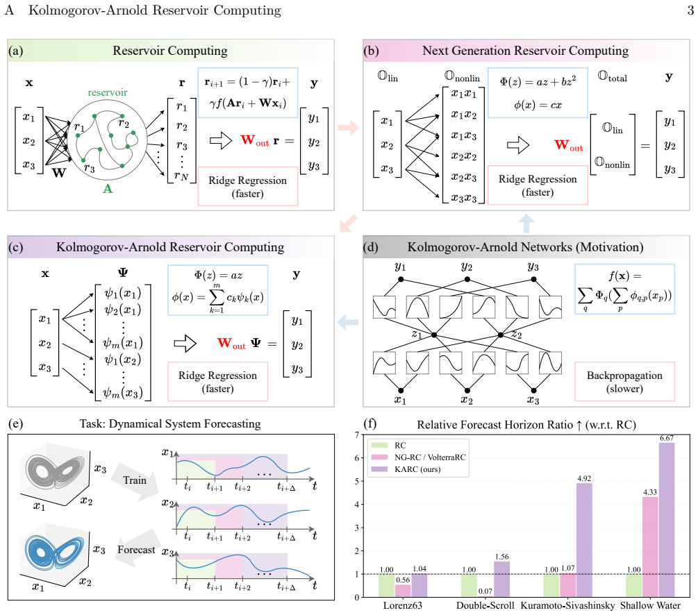
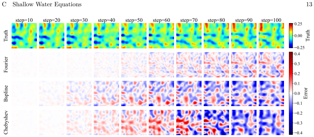
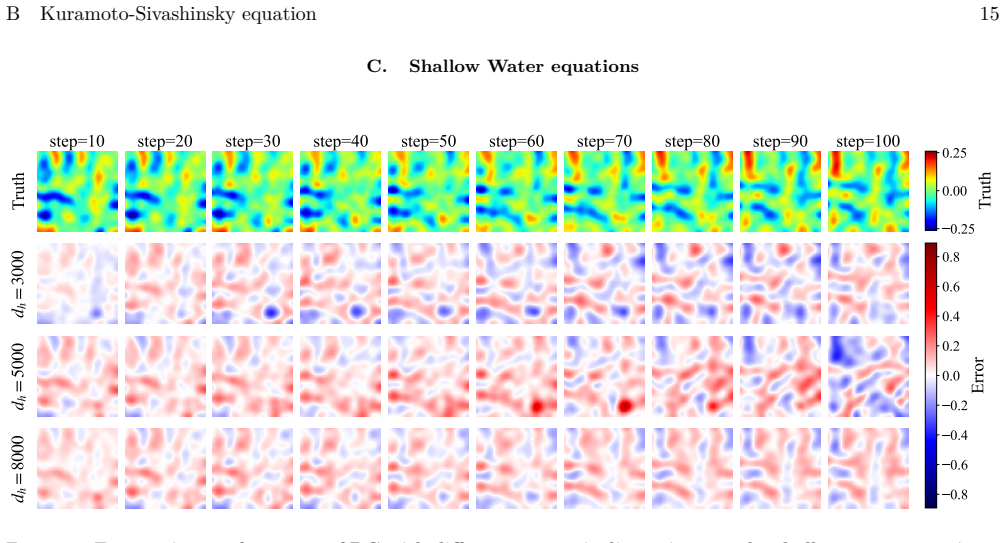
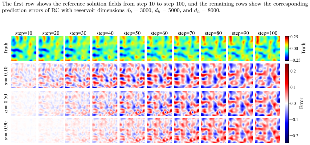
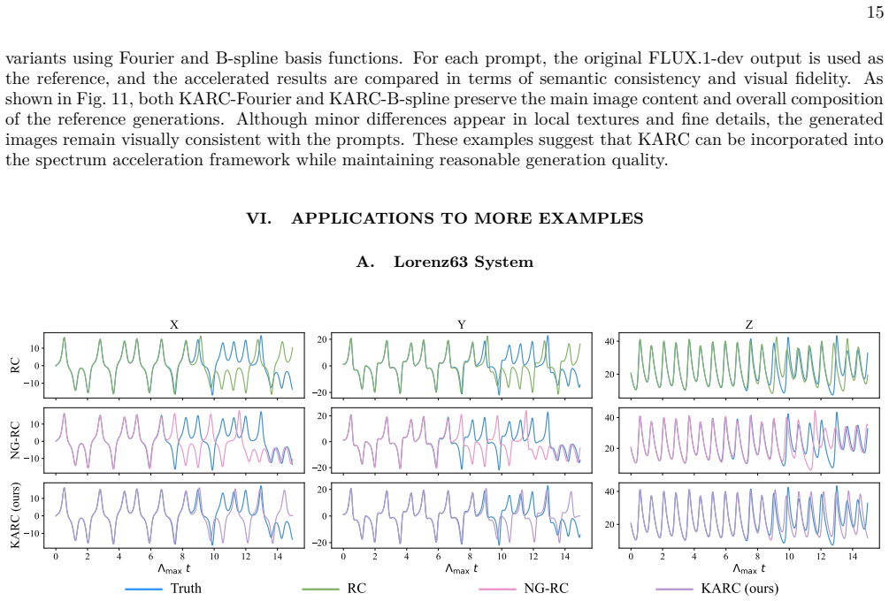
KARC replaces reservoirs with explicit basis-function expansions inspired by the Kolmogorov-Arnold representation theorem. We rigorously show that KARC is a lightweight design of Kolmogorov-Arnold networks (KANs), preserving the potential expressive capacity of KANs while admitting efficient closed-form training of reservoir computing. At comparable cost, KARC outperforms existing reservoir computing methods on challenging benchmarks including partial differential equations. It can also be integrated with generative diffusion models for text-to-image generation.
What carries the argument
Explicit basis-function expansions inspired by the Kolmogorov-Arnold representation theorem, used in place of recurrent reservoirs to carry the network's representational capacity.
If this is right
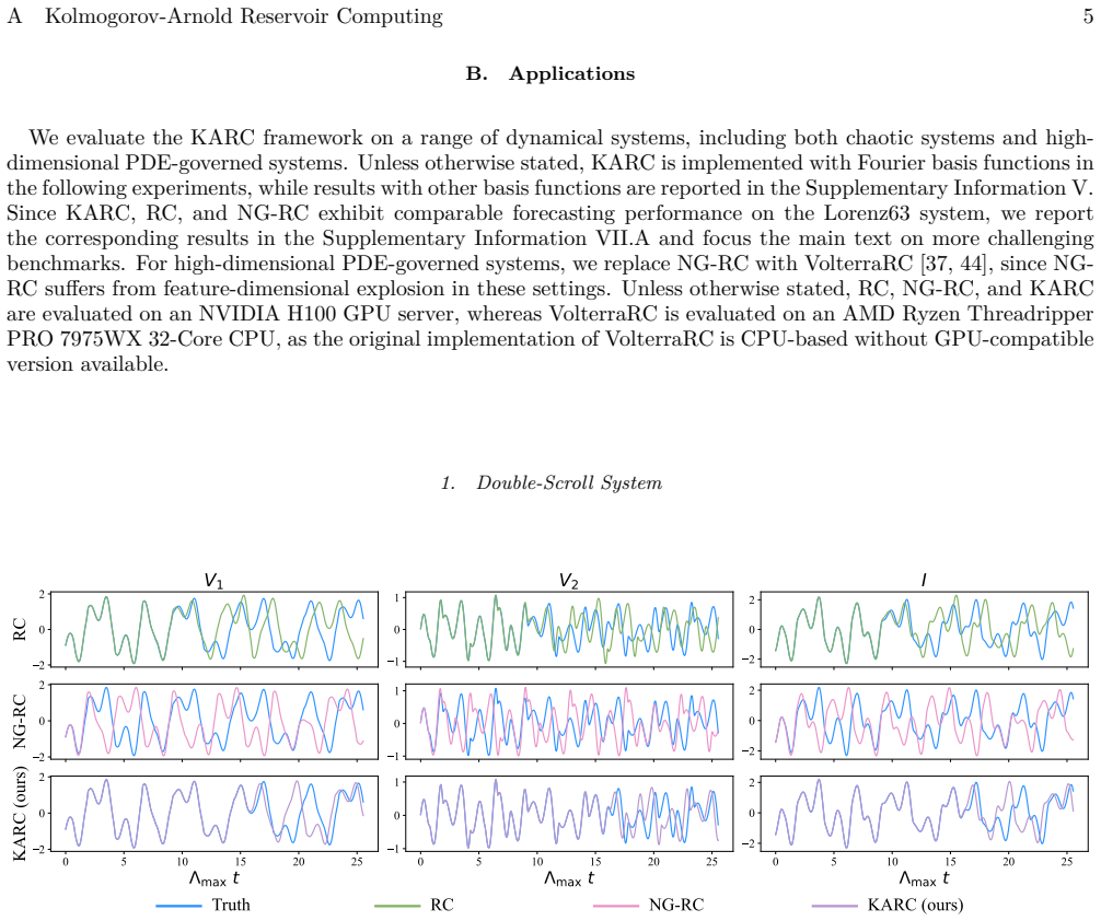
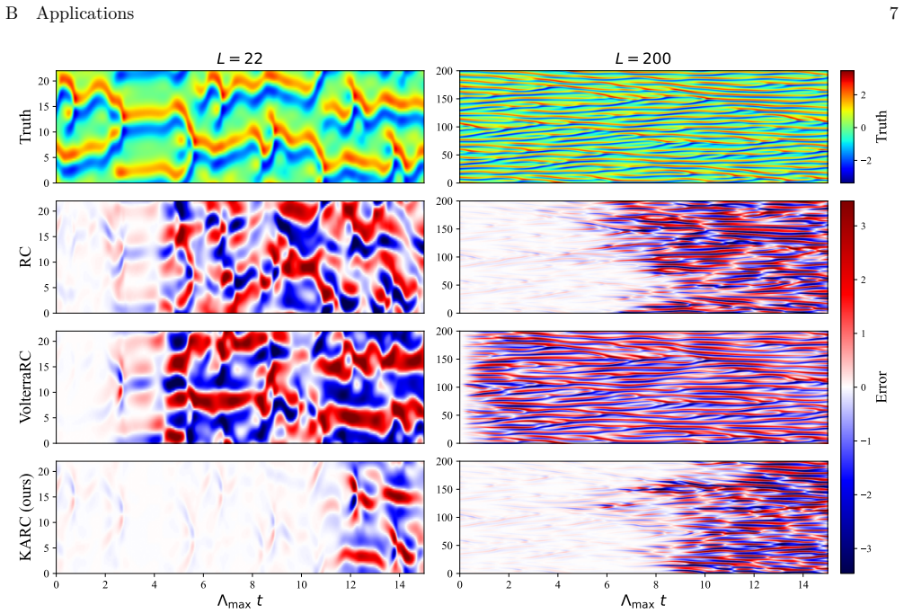
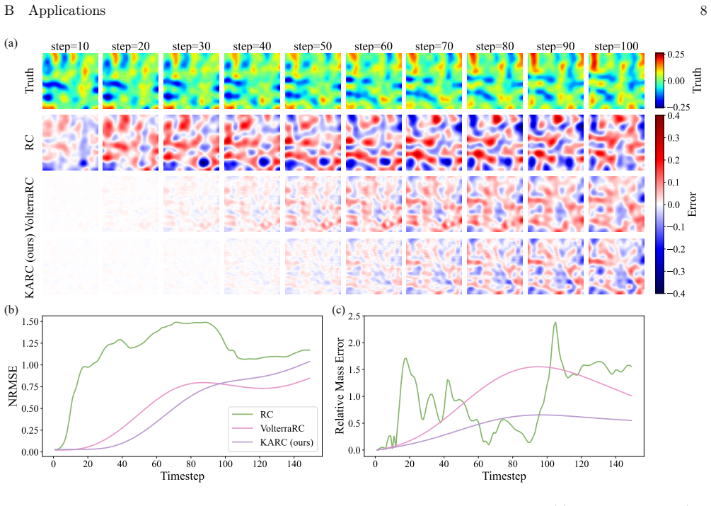
- At comparable cost, KARC outperforms existing reservoir computing methods on challenging benchmarks including partial differential equations.
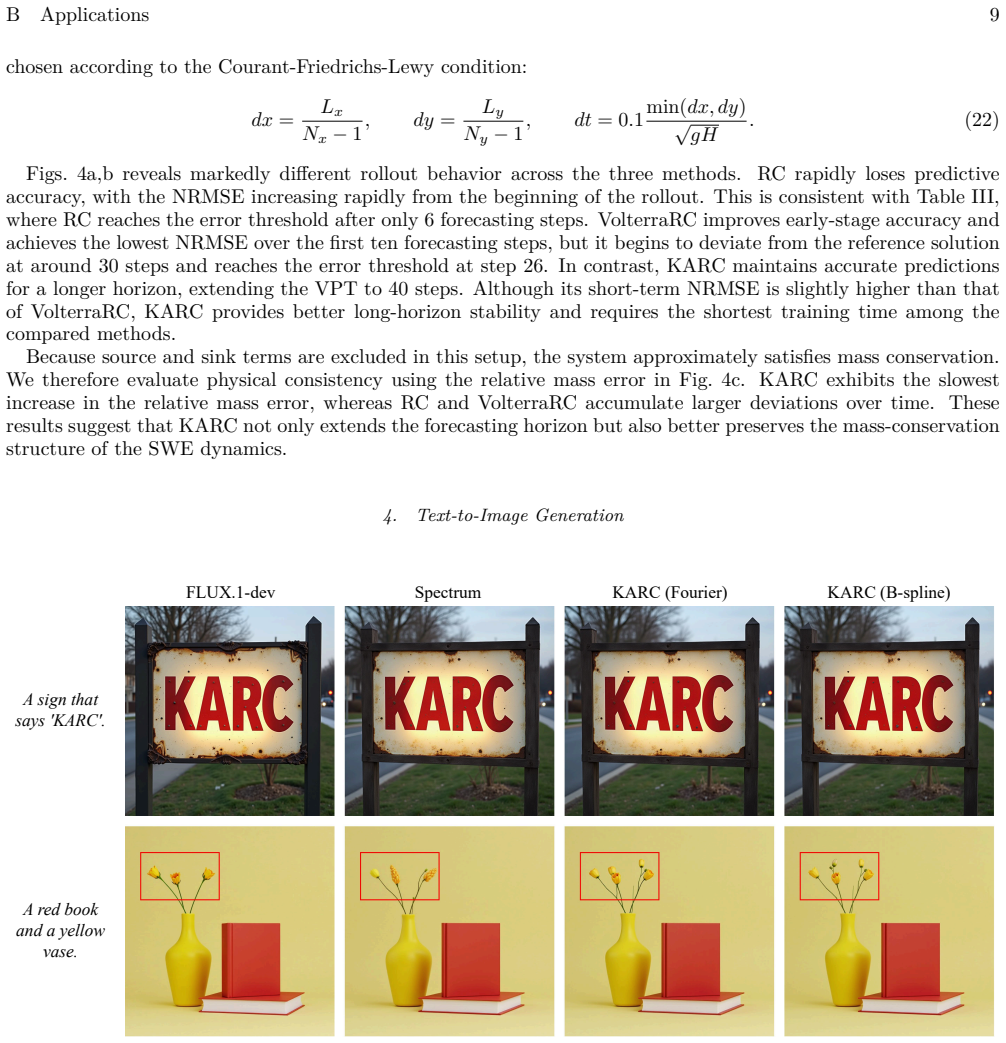
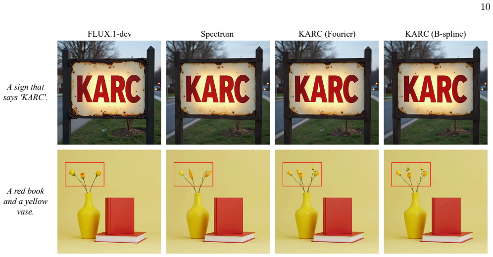
- It can be integrated with generative diffusion models for text-to-image generation.
- This establishes a principled bridge between reservoir computing and KANs, enabling efficient and high-fidelity dynamical system forecasting.
Where Pith is reading between the lines
- The same basis expansions could be tested as drop-in replacements in other recurrent architectures that currently rely on random or trained reservoirs.
- Because training remains closed-form, KARC may scale more readily to very long time series than gradient-based KAN variants.
- Integration with diffusion models opens the possibility of using KARC as a temporal prior inside generative pipelines for physics-informed image or video synthesis.
Load-bearing premise
The basis-function expansions inspired by the Kolmogorov-Arnold representation theorem can be substituted for conventional reservoirs without loss of the expressive capacity that KANs are claimed to possess.
What would settle it
A benchmark dynamical system on which KARC matches or exceeds full KAN performance in accuracy yet requires substantially more parameters or training time than standard reservoir methods would falsify the efficiency-plus-capacity claim.
Figures


read the original abstract
Reservoir computing offers a lightweight framework for forecasting dynamical systems but may struggle to capture long-range dependencies due to limited representational capacity. Conventional reservoir computing recurrently uses trainable reservoirs with hyperparameter sensitivity, while the next-generation reservoir computing removes recurrence at the cost of rapidly growing feature dimensions. Here, we develop Kolmogorov-Arnold Reservoir Computing (KARC), which replaces reservoirs with explicit basis-function expansions inspired by the Kolmogorov-Arnold representation theorem. We rigorously show that KARC is a lightweight design of Kolmogorov-Arnold networks (KANs), preserving the potential expressive capacity of KANs while admitting efficient closed-form training of reservoir computing. At comparable cost, KARC outperforms existing reservoir computing methods on challenging benchmarks including partial differential equations. It can also be integrated with generative diffusion models for text-to-image generation. This work thus establishes a principled bridge between reservoir computing and KANs, enabling efficient and high-fidelity dynamical system forecasting.
Editorial analysis
A structured set of objections, weighed in public.
Referee Report
Summary. The manuscript introduces Kolmogorov-Arnold Reservoir Computing (KARC), which substitutes explicit basis-function expansions inspired by the Kolmogorov-Arnold representation theorem for conventional reservoirs in reservoir computing. It claims KARC is a lightweight design of Kolmogorov-Arnold networks (KANs) that preserves their expressive capacity while enabling efficient closed-form training, outperforms existing RC methods on dynamical-system benchmarks including PDEs at comparable cost, and integrates with generative diffusion models.
Significance. If the central claims of preserved expressive capacity and rigorous closed-form training hold, the work would establish a useful bridge between reservoir computing and KANs, offering a principled route to efficient, high-fidelity forecasting of dynamical systems with potential impact in scientific machine learning.
major comments (1)
- Abstract: the claim of a 'rigorous' demonstration that KARC preserves the expressive capacity of KANs is load-bearing for the central contribution, yet the provided material supplies no derivation, theorem statement, or proof outline; without explicit verification of this step the superiority and preservation assertions cannot be assessed.
Simulated Author's Rebuttal
We thank the referee for their review and for highlighting this critical point about the central claim. We address the comment below and commit to a revision that supplies the missing supporting material.
read point-by-point responses
-
Referee: Abstract: the claim of a 'rigorous' demonstration that KARC preserves the expressive capacity of KANs is load-bearing for the central contribution, yet the provided material supplies no derivation, theorem statement, or proof outline; without explicit verification of this step the superiority and preservation assertions cannot be assessed.
Authors: We agree the abstract's assertion requires explicit verification. The current manuscript states the claim at a high level in Section 3 but does not include a formal theorem or proof outline. In the revised manuscript we will insert a new subsection (Section 3.2) containing: (i) the theorem statement that KARC constitutes a lightweight KAN design preserving expressive capacity via finite Kolmogorov-Arnold basis expansions in the reservoir, and (ii) a concise proof sketch relying on the universal approximation property of KANs together with the closed-form linear readout. This addition will allow direct assessment of the preservation argument and the closed-form training claim. revision: yes
Circularity Check
No significant circularity
full rationale
The paper's central claim is that KARC replaces conventional reservoirs with explicit basis-function expansions drawn from the Kolmogorov-Arnold theorem, yielding a lightweight KAN variant that supports closed-form training while preserving expressive capacity. This construction is presented as an independent design choice whose equivalence to KANs is asserted via a rigorous demonstration rather than by redefining the target quantity in terms of itself or by fitting parameters to the very quantities being predicted. No self-citation chain is invoked as the sole justification for a uniqueness theorem, no fitted input is relabeled as a prediction, and no ansatz is smuggled through prior self-work. The derivation therefore remains self-contained against external benchmarks and does not reduce to its inputs by construction.
Axiom & Free-Parameter Ledger
axioms (1)
- standard math The Kolmogorov-Arnold representation theorem applies to the explicit basis-function expansions used in place of reservoirs.
Reference graph
Works this paper leans on
-
[1]
Lim and S
B. Lim and S. Zohren, Time-series forecasting with deep learning: a survey, Philos. Trans. R. Soc. A Math. Phys. Eng. Sci. 379, 20200209 (2021)
2021
-
[2]
Kovachki, Z
N. Kovachki, Z. Li, B. Liu, K. Azizzadenesheli, K. Bhattacharya, A. Stuart, and A. Anandkumar, Neural operator: Learning maps between function spaces with applications to PDEs, J. Mach. Learn. Res. 24, 1 (2023)
2023
-
[3]
Empirical Evaluation of Gated Recurrent Neural Networks on Sequence Modeling
J. Chung, C. Gulcehre, K. Cho, and Y. Bengio, Empirical evaluation of gated recurrent neural networks on sequence modeling, arXiv preprint arXiv:1412.3555 (2014)
work page internal anchor Pith review Pith/arXiv arXiv 2014
-
[4]
Vaswani, N
A. Vaswani, N. Shazeer, N. Parmar, J. Uszkoreit, L. Jones, A. N. Gomez, Ł. Kaiser, and I. Polosukhin, Attention is all you need, in Advances in Neural Information Processing Systems , Vol. 30 (2017) pp. 5998–6008
2017
-
[5]
Z. Li, N. B. Kovachki, K. Azizzadenesheli, B. liu, K. Bhattacharya, A. Stuart, and A. Anandkumar, Fourier neural operator for parametric partial differential equations, in Int. Conf. Learn. Represent. (2021)
2021
-
[6]
Wang and C
T. Wang and C. Wang, Latent neural operator for solving forward and inverse PDE problems, in Adv. Neural Inf. Process. Syst., Vol. 37 (2024)
2024
-
[7]
L. Lu, P. Jin, G. Pang, Z. Zhang, and G. E. Karniadakis, Learning nonlinear operators via DeepONet based on the universal approximation theorem of operators, Nat. Mach. Intell. 3, 218 (2021)
2021
-
[8]
Goswami, A
S. Goswami, A. Bora, Y. Yu, and G. E. Karniadakis, Physics-informed deep neural operator networks, in Machine Learning in Modeling and Simulation: Methods and Applications , Computational Methods in Engineering & the Sciences, edited by T. Rabczuk and K.-J. Bathe (Springer, 2023) pp. 219–254
2023
-
[9]
N. B. Kovachki, S. Lanthaler, and A. M. Stuart, Operator learning: Algorithms and analysis, in Numerical Analysis Meets Machine Learning , Handb. Numer. Anal., Vol. 25 (Elsevier, 2024) pp. 419–467
2024
-
[10]
S. Liu, Y. Yu, T. Zhang, H. Liu, X. Liu, and D. Meng, Architectures, variants, and performance of neural operators: A comparative review, Neurocomputing 648, 130518 (2025)
2025
-
[11]
Benidis, S
K. Benidis, S. S. Rangapuram, V. Flunkert, Y. Wang, D. Maddix, C. Turkmen, J. Gasthaus, M. Bohlke-Schneider, D. Salinas, L. Stella, et al. , Deep learning for time series forecasting: Tutorial and literature survey, ACM Comput. Surv. 55, 1 (2022)
2022
-
[13]
Pathak, B
J. Pathak, B. Hunt, M. Girvan, Z. Lu, and E. Ott, Model-free prediction of large spatiotemporally chaotic systems from data: A reservoir computing approach, Phys. Rev. Lett. 120, 024102 (2018)
2018
-
[15]
N. Lin, S. Wang, Y. Li, B. Wang, S. Shi, Y. He, W. Zhang, Y. Yu, Y. Zhang, X. Zhang, et al. , Resistive memory-based zero-shot liquid state machine for multimodal event data learning, Nat. Comput. Sci. 5, 37 (2025)
2025
-
[16]
R. S. Zimmermann and U. Parlitz, Observing spatio-temporal dynamics of excitable media using reservoir computing, Chaos 28, 043118 (2018)
2018
-
[17]
Xiong and H
Y. Xiong and H. Zhao, Chaotic time series prediction based on long short-term memory neural networks, Sci. China Phy. Mech. Astron. 49, 120501 (2019)
2019
-
[18]
H. Fan, J. Jiang, C. Zhang, X. Wang, and Y.-C. Lai, Long-term prediction of chaotic systems with machine learning, Phys. Rev. Res. 2, 012080 (2020)
2020
-
[19]
Rafayelyan, J
M. Rafayelyan, J. Dong, Y. Tan, F. Krzakala, and S. Gigan, Large-scale optical reservoir computing for spatiotemporal chaotic systems prediction, Phys. Rev. X 10, 041037 (2020)
2020
-
[20]
Z. Lin, Z. Lu, Z. Di, and Y. Tang, Learning noise-induced transitions by multi-scaling reservoir computing, Nat. Commun. 15, 6584 (2024)
2024
-
[21]
H. Tan, L. Shi, S. Wang, and S.-X. Qu, Improving model-free prediction of chaotic dynamics by purifying the incomplete input, AIP Adv. 14 (2024)
2024
-
[22]
X. Li, Q. Zhu, C. Zhao, X. Duan, B. Zhao, X. Zhang, H. Ma, J. Sun, and W. Lin, Higher-order granger reservoir D Error Bound of KARC for Fading Memory Dynamical Systems 22 computing: simultaneously achieving scalable complex structures inference and accurate dynamics prediction, Nat. Commun. 15, 2506 (2024)
2024
-
[23]
X. Han, Z. Qi, V. Kundrat, H. Li, Z. Li, X. Guo, P. Mao, W. Zheng, S. Hou, R. Liu, et al. , Very-large-scale mimetic optogenetic synapses for physical reservoir computing, Nat. Commun. 17, 1514 (2026)
2026
-
[24]
Amann, K
A. Amann, K. Lüdge, U. Parlitz, and M. Small, Nonlinear dynamics of reservoir computing: Theory, realization, and application, Chaos 36 (2026)
2026
-
[25]
Grigoryeva and J.-P
L. Grigoryeva and J.-P. Ortega, Universal discrete-time reservoir computers with stochastic inputs and linear readouts using non-homogeneous state-affine systems, J. Mach. Learn. Res. 19, 1 (2018)
2018
-
[26]
Grigoryeva and J.-P
L. Grigoryeva and J.-P. Ortega, Echo state networks are universal, Neural Netw. 108, 495 (2018)
2018
-
[27]
Gonon and J.-P
L. Gonon and J.-P. Ortega, Reservoir computing universality with stochastic inputs, IEEE Trans. Neural Netw. Learn. Syst. 31, 100 (2019)
2019
-
[28]
A. Hart, J. Hook, and J. Dawes, Embedding and approximation theorems for echo state networks, Neural Netw. 128, 234 (2020)
2020
-
[29]
Gonon and J.-P
L. Gonon and J.-P. Ortega, Fading memory echo state networks are universal, Neural Netw. 138, 10 (2021)
2021
-
[30]
L. A. Thiede and U. Parlitz, Gradient based hyperparameter optimization in echo state networks, Neural Netw. 115, 23 (2019)
2019
-
[31]
Ren and H
B. Ren and H. Ma, Global optimization of hyper-parameters in reservoir computing, Electron. Res. Arch. 30, 2719 (2022)
2022
-
[32]
M. Yan, C. Huang, P. Bienstman, P. Tino, W. Lin, and J. Sun, Emerging opportunities and challenges for the future of reservoir computing, Nat. Commun. 15, 2056 (2024)
2056
-
[33]
Lukoševičius and H
M. Lukoševičius and H. Jaeger, Reservoir computing approaches to recurrent neural network training, Comput. Sci. Rev. 3, 127 (2009)
2009
-
[34]
Martin and C
E. Martin and C. Cundy, Parallelizing linear recurrent neural nets over sequence length, in Int. Conf. Learn. Represent. (2018)
2018
-
[35]
D. J. Gauthier, E. Bollt, A. Griffith, and W. A. S. Barbosa, Next generation reservoir computing, Nat. Commun. 12, 5564 (2021)
2021
-
[37]
Grigoryeva, H
L. Grigoryeva, H. L. J. Ting, and J.-P. Ortega, Infinite-dimensional next-generation reservoir computing, Phys. Rev. E 111, 035305 (2025)
2025
-
[38]
Cestnik and E
R. Cestnik and E. A. Martens, Next-generation reservoir computing for dynamical inference, Chaos 36, 013115 (2026)
2026
-
[39]
A. N. Kolmogorov, On the representation of continuous functions of many variables by superposition of continuous functions of one variable and addition, Dokl. Akad. Nauk SSSR 114, 953 (1957)
1957
-
[40]
Z. Liu, Y. Wang, S. Vaidya, F. Ruehle, J. Halverson, M. Soljačić, T. Y. Hou, and M. Tegmark, KAN: Kolmogorov-arnold networks, in Proceedings of the International Conference on Learning Representations (2025)
2025
-
[41]
Z. Liu, M. Tegmark, P. Ma, W. Matusik, and Y. Wang, Kolmogorov-arnold networks meet science, Phys. Rev. X 15, 041051 (2025)
2025
-
[42]
MesaNet: Sequence Modeling by Locally Optimal Test-Time Training
J. von Oswald, N. Scherrer, S. Kobayashi, L. Versari, S. Yang, M. Schlegel, K. Maile, Y. Schimpf, O. Sieberling, A. Meulemans, et al. , Mesanet: Sequence modeling by locally optimal test-time training, arXiv:2506.05233 (2025)
work page internal anchor Pith review Pith/arXiv arXiv 2025
-
[43]
J. Han, J. Shi, P. Li, H. Ye, Q. Guo, and S. Ermon, Adaptive spectral feature forecasting for diffusion sampling acceleration, in Proceedings of the IEEE/CVF Conference on Computer Vision and Pattern Recognition (2026) pp. 43320–43330
2026
-
[44]
Gonon, L
L. Gonon, L. Grigoryeva, and J.-P. Ortega, Reservoir kernels and volterra series, IEEE Trans. Neural Netw. Learn. Syst. , 1 (2025)
2025
-
[45]
G. K. Vallis, Atmospheric and Oceanic Fluid Dynamics: Fundamentals and Large-Scale Circulation , 2nd ed. (Cambridge University Press, 2017)
2017
-
[47]
G. Li, L. Huang, and Y. Lei, Reservoir computing meeting kolmogorov-arnold networks: prediction of high-dimensional chaotic systems, Chaos 35, 103120 (2025)
2025
-
[48]
Z. Lin, J. Kurths, and Y. Tang, Multi-scaling reservoir computing learns noise-induced transitions with Lévy noise, Chaos 35, 073132 (2025)
2025
-
[49]
Raissi, P
M. Raissi, P. Perdikaris, and G. E. Karniadakis, Physics-informed neural networks: a deep learning framework for solving forward and inverse problems involving nonlinear partial differential equations, J. Comput. Phys. 378, 686 (2019)
2019
-
[50]
Z. Li, H. Zheng, N. Kovachki, D. Jin, H. Chen, B. Liu, K. Azizzadenesheli, and A. Anandkumar, Physics-informed neural operator for learning partial differential equations, ACM/IMS J. Data Sci. 1, 1 (2024) . Supplementary Information: Kolmogorov-Arnold Reservoir Computing Juntian Huang, 1 Jürgen Kurths, 2, 3, 4 and Ying Tang 1, 5, 6, 7, ∗ 1Institute of Fun...
2024
-
[51]
D. J. Gauthier, E. Bollt, A. Griffith, and W. A. S. Barbosa, Next generation reservoir computing, Nat. Commun. 12, 5564 (2021)
2021
-
[52]
Grigoryeva, H
L. Grigoryeva, H. L. J. Ting, and J.-P. Ortega, Infinite-dimensional next-generation reservoir computing, Phys. Rev. E 111, 035305 (2025)
2025
-
[53]
echo state
H. Jaeger, The “echo state” approach to analysing and training recurrent neural networks–with an erratum note , GMD Technical Report 148 (German National Research Center for Information Technology, Bonn, Germany, 2001)
2001
-
[54]
Maass, T
W. Maass, T. Natschläger, and H. Markram, Real-time computing without stable states: A new framework for neural computation based on perturbations, Neural Comput. 14, 2531 (2002)
2002
-
[55]
E. Bollt, On explaining the surprising success of reservoir computing forecaster of chaos? the universal machine learning dynamical system with contrast to var and dmd, Chaos 31, 013108 (2021)
2021
-
[56]
Black Forest Labs, FLUX, https://github.com/black-forest-labs/flux (2024), gitHub repository
2024
-
[57]
J. Han, J. Shi, P. Li, H. Ye, Q. Guo, and S. Ermon, Adaptive spectral feature forecasting for diffusion sampling accelera- tion, in Proceedings of the IEEE/CVF Conference on Computer Vision and Pattern Recognition (2026) pp. 43320–43330
2026
-
[58]
Z. Li, N. B. Kovachki, K. Azizzadenesheli, B. liu, K. Bhattacharya, A. Stuart, and A. Anandkumar, Fourier neural operator for parametric partial differential equations, in Int. Conf. Learn. Represent. (2021)
2021
discussion (0)
Sign in with ORCID, Apple, or X to comment. Anyone can read and Pith papers without signing in.