Reducing measurement error with adaptivity
Pith reviewed 2026-06-26 14:16 UTC · model grok-4.3
The pith
Adaptive measurement circuits can reduce errors in noisy qubit measurements better than any non-adaptive circuit with the same number of measurements.
A machine-rendered reading of the paper's core claim, the machinery that carries it, and where it could break.
Core claim
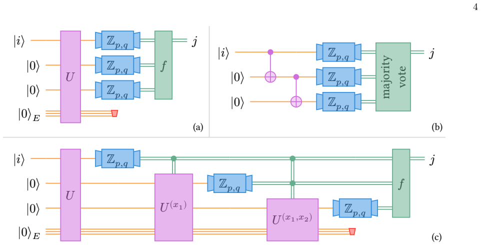
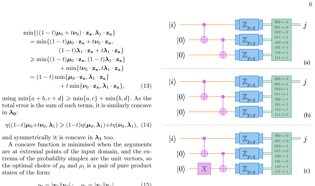
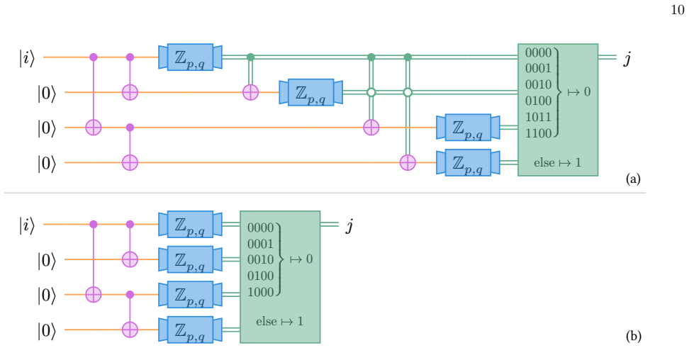
We show that adaptivity, also called feed-forward, is a powerful resource in reducing the error of measurement circuits that combine multiple uses of a noisy measuring device. Adaptive measurement circuits can in general reduce overall measurement errors further than any non-adaptive measurement circuit could with the same number of measurements. In particular, for a large class of noisy two-outcome qubit measurements, such an adaptive advantage can exist when as few as three measurements are used. We also show that the adaptive advantage is unbounded across the class of noisy two-outcome qubit measurements, as the number of uses of the device increases.
What carries the argument
Adaptive measurement circuits with feed-forward, in which the results of previous measurements influence the choice of further measurements and processing.
If this is right
- Methods exist for finding optimal measurement circuits in both adaptive and non-adaptive cases.
- An adaptive advantage exists for a large class of noisy two-outcome qubit measurements at three uses.
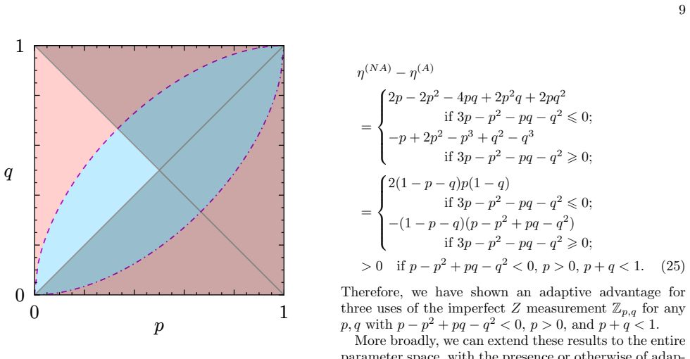
- The adaptive advantage is unbounded as the number of uses of the device increases.
- General results on the limits of such circuits apply to measuring a qubit and more generally a qudit.
Where Pith is reading between the lines
- Similar adaptive advantages might exist for other types of quantum measurements or systems beyond the specified class.
- The optimal circuit finding methods could be applied to design better protocols in quantum computing tasks.
Load-bearing premise
The existence of a large class of noisy two-outcome qubit measurements for which the adaptive advantage holds at three uses, making the class representative for the general statements.
What would settle it
A concrete noisy two-outcome qubit measurement where the lowest error with any three-measurement adaptive circuit is no better than with the best non-adaptive circuit.
Figures


read the original abstract
We show that adaptivity, also called feed-forward, is a powerful resource in reducing the error of measurement circuits that combine multiple uses of a noisy measuring device. In previous work, it has been shown that error in measurements can be mitigated by using the measuring device multiple times. So far, the most effective protocols have been parallel measurement schemes, where all measurements are simultaneous. We extend this idea to adaptive measurement schemes, where the results of previous measurements can influence our choice of processing further down the circuit. We show that adaptive measurement circuits can in general reduce overall measurement errors further than any non-adaptive measurement circuit could with the same number of measurements. In particular, we show that for a large class of noisy two-outcome qubit measurements, such an adaptive advantage can exist when as few as three measurements are used. We also show that the adaptive advantage is unbounded across the class of noisy two-outcome qubit measurements, as the number of uses of the device increases. As part of this work, we devise and use methods for finding optimal measurement circuits in both the non-adaptive and adaptive cases. In addition, we prove general results about the limits of such circuits, both in measuring a qubit, and more generally, a qudit.
Editorial analysis
A structured set of objections, weighed in public.
Referee Report
Summary. The manuscript claims that adaptive (feed-forward) measurement circuits outperform non-adaptive ones in reducing overall error for the same number of uses of a noisy device. For a large class of noisy two-outcome qubit measurements, an adaptive advantage exists already at three uses; the advantage is unbounded as the number of uses grows. The authors supply explicit constructions, methods for finding optimal adaptive and non-adaptive circuits, and general bounds that apply both to qubits and to qudits.
Significance. If the constructions and comparisons hold, the work establishes adaptivity as a concrete resource for measurement-error mitigation beyond what parallel schemes achieve. The n=3 explicit advantage and the unboundedness result across a broad noise class, together with the optimization methods, would be useful contributions to quantum information processing.
major comments (2)
- [Theorem/Construction for n=3 (likely §4 or §5)] The central existence claim for the adaptive advantage at n=3 rests on an unspecified 'large class' of noisy two-outcome qubit measurements. Without an explicit, checkable definition of this class (e.g., the precise noise model or parameter range in the relevant theorem), it is impossible to verify that the stated constructions indeed lie inside the class and that the comparison to the optimal non-adaptive circuit is correctly performed.
- [Unboundedness result (likely §6)] The unboundedness statement as n increases likewise depends on the same class definition. If the class is defined only implicitly via the existence of the constructions, the claim risks being circular; an independent characterization of the noise family is needed to confirm the result is not tautological.
minor comments (2)
- [Methods for optimal circuits] Notation for the adaptive circuit (feed-forward maps, decision trees) should be introduced with a small diagram or explicit pseudocode in the methods section to make the optimality-finding algorithm reproducible.
- [General results for qudits] The general qudit bounds are stated without an accompanying example or numerical check; adding one small qudit instance would clarify the scope.
Simulated Author's Rebuttal
We thank the referee for their careful reading and constructive comments. We address the major comments point by point below. The concerns raised are valid regarding clarity, and we will revise the manuscript to provide an explicit, independent definition of the noise class.
read point-by-point responses
-
Referee: [Theorem/Construction for n=3 (likely §4 or §5)] The central existence claim for the adaptive advantage at n=3 rests on an unspecified 'large class' of noisy two-outcome qubit measurements. Without an explicit, checkable definition of this class (e.g., the precise noise model or parameter range in the relevant theorem), it is impossible to verify that the stated constructions indeed lie inside the class and that the comparison to the optimal non-adaptive circuit is correctly performed.
Authors: We agree that the definition requires greater explicitness for independent verification. The class is characterized by a specific noise model on two-outcome qubit measurements (POVMs with a tunable bias parameter in a defined interval), but the presentation in the theorems may not make the membership conditions immediately checkable. In the revised manuscript we will insert a dedicated paragraph or subsection that states the precise noise model, the parameter range, and the conditions under which the n=3 constructions belong to the class and outperform the optimal non-adaptive circuit. revision: yes
-
Referee: [Unboundedness result (likely §6)] The unboundedness statement as n increases likewise depends on the same class definition. If the class is defined only implicitly via the existence of the constructions, the claim risks being circular; an independent characterization of the noise family is needed to confirm the result is not tautological.
Authors: The class is defined by the noise model and parameter range independently of any particular construction; the constructions are then shown to lie inside that class while achieving growing advantage. Nevertheless, the referee's observation that the current wording risks appearing circular is fair. We will revise §6 (and the preceding sections) to first state the class definition in full, then present the family of constructions and the general bounds that establish unbounded advantage within that independently defined class. revision: yes
Circularity Check
No significant circularity detected
full rationale
The paper establishes its central claims through explicit constructions of adaptive and non-adaptive measurement circuits, direct comparisons of their error performance on a specified class of noisy two-outcome qubit measurements, and methods for identifying optimal circuits in both settings. These elements are presented as independent contributions that enable the stated advantage at n=3 and its unbounded growth, without any reduction of predictions to fitted inputs, self-definitional equivalences, or load-bearing self-citations that collapse the argument to prior unverified results by the same authors. The derivation chain remains self-contained against external benchmarks via the explicit constructions and general limit proofs.
Axiom & Free-Parameter Ledger
Reference graph
Works this paper leans on
-
[1]
|𝑖⟩ 𝕄SIC 𝑗 |0⟩ 𝕄SIC |0⟩ 𝕄SIC 𝒜︀ 𝑓 ℬ︀(𝑥1𝑥2) FIG
The total error achieved by this circuit is 1 2 − √ 3 6 = 0.211..., while the minimal non-adaptive total error is 1 4 = 0.25. |𝑖⟩ 𝕄SIC 𝑗 |0⟩ 𝕄SIC |0⟩ 𝕄SIC 𝒜︀ 𝑓 ℬ︀(𝑥1𝑥2) FIG. 21. For three uses ofM SIC, rather than finding an optimal non-adaptive circuit, we find it is easier to find an optimal circuit of the form shown, where the third measurement is perf...
-
[2]
and ( 1 2 ,0). Therefore, we need only consider: ε(x1x2) 0 , ε(x1x2) 1 ∈ n 0, 1 2 , 1 2 ,0 , 1 2 1− 1√ 3 , 1 2 1− 1√ 3 o .(87) We thus have three options for what to do for each (x1, x2)∈[4] 2, meaning that we have 3 42 = 3 16 pos- sibilities to check in total, or about 43 million. This is a vast improvement over 2 64, and can be done by ex- haustive sear...
-
[3]
In combination with (83), we thus obtain: η(NA)(MSIC,3) = 1 8 = 1 23 .(88) Then, for any oddNgreater than or equal to 5, we con- sider doing an adaptive circuit consisting of one measure- ment ofM ⊗(N−3) SIC , followed by one ofM ⊗3 SIC adaptively. By a similar method to Proposition 3, the eventual to- tal error must be lower bounded by the product of the...
-
[4]
In fact, we can use a POVM in any dimension (referred to ashearlier), even if the measurement we are attempting to approximate remains the projective Zmeasurement on a qubit
The generalised symmetric imperfectZ All of the examples we have been using so far are qubit measurements, but the mathematics doesn’t limit us to just these. In fact, we can use a POVM in any dimension (referred to ashearlier), even if the measurement we are attempting to approximate remains the projective Zmeasurement on a qubit. We will still suppose t...
-
[5]
Moreover, we can take theA k to be isometries, map- ping|0⟩ ⟨0|and|1⟩ ⟨1|to distinct computational basis states |i0⟩ ⟨i0|and|i 1⟩ ⟨i1|. By the symmetry ofS m,t, we can take |i0⟩ ⟨i0|=|0⟩ ⟨0|,|i 1⟩ ⟨i1|=|1⟩ ⟨1|without loss of generality, since any other such isometry is equivalent up to a per- mutation before and after the measurementS m,t. This tells us e...
-
[6]
Proof.See Appendix D 9
Then: P Bin(n, p)⩾ 1 2 n ⩽ 2 p p(1−p) n ,(98) whereBin(n, p)is the binomial distribution withntrials and probability of successp. Proof.See Appendix D 9. 24 We can turn this into a result about particular multino- mial distributions, mirroring the distribution we get from measuring generalised symmetric imperfectZ: Lemma 10.LetXbe a random variable with d...
-
[7]
First, we will takep=q < 1 2, so we only consider symmetric imper- fectZmeasurements
ImperfectZ For the imperfectZmeasurement (1), we will upper boundη (NA) d by constructing a non-adaptive circuit, al- though we will require a couple of concessions. First, we will takep=q < 1 2, so we only consider symmetric imper- fectZmeasurements. Secondly, we assume thatN= 2 dn is a multiple of 2 d, as the circuit we have chosen to anal- yse will req...
-
[8]
First, consider what a single trine measurement can do
The trine For the trine (72), we’ll construct an adaptive circuit, giving an upper bound onη (A) d . First, consider what a single trine measurement can do. Suppose we partition [d] into three setsA, B, C⊆[d] withA⊔B⊔C= [d], and define a channelAwith: A:|i⟩ ⟨i| 7→ ψ⊥ 0 ψ⊥ 0 ifi∈A; ψ⊥ 1 ψ⊥ 1 ifi∈B; ψ⊥ 2 ψ⊥ 2 ifi∈C. (139) where ψ⊥ 0 =|1⟩, ψ⊥ 1 = √ 3...
-
[9]
The qubit SIC-POVM Given its similar definition to the trine, with all POVM elements being rank one, it perhaps comes as little sur- prise that we can make a similar argument for the qubit SIC-POVM (75), and construct an adaptive circuit to up- per boundη (A) d . To be specific, if we have a partition of [d] into four setsA, B, C, D⊆[d] withA⊔B⊔C⊔D= [d], ...
-
[10]
The generalised symmetric imperfectZ Our first example in this section was the symmetric im- perfectZ. We have noted before that the generalised symmetric imperfectZ(92) is a generalisation of this (Zp,p =S 2,p), so for generalS m,t, we will try to use a similar non-adaptive circuit to boundη (NA) d . We will as- sume thatt < m−1 m (so that the likeliest ...
-
[11]
Y. Guryanova, N. Friis, and M. Huber, Ideal projec- tive measurements have infinite resource costs, Quantum https://doi.org/10.22331/q-2020-01-13-222 (2020)
-
[12]
E. Haapasalo, T. Heinosaari, and Y. Kuramochi, Saturation of repeated quantum measurements, Jour- nal of Physics A: Mathematical and Theoretical https://doi.org/10.1088/1751-8113/49/33/33LT01 (2016)
-
[13]
T. Bullock and T. Heinosaari, Quantum state discrim- ination via repeated measurements and the rule of three, Quantum Studies: Mathematics and Foundations https://doi.org/10.1007/s40509-020-00233-7 (2021)
-
[14]
J. M. G¨ unther, F. Tacchino, J. R. Wootton, I. Tav- ernelli, and P. K. Barkoutsos, Improving readout in quantum simulations with repetition codes, Quantum Science and Technology https://doi.org/10.1088/2058- 9565/ac3386 (2021)
-
[15]
R. Hicks, B. Kobrin, C. W. Bauer, and B. Nach- man, Active readout-error mitigation, Physical Review A https://doi.org/10.1103/PhysRevA.105.012419 (2022)
-
[16]
N. Linden and P. Skrzypczyk, How to use arbitrary mea- suring devices to perform almost-perfect measurements, Physical Review A https://doi.org/10.1103/8tph-mc2p (2025)
-
[17]
C. Corlett, I. ˇCepait˙ e, A. J. Daley, C. Gustiani, et al., Speeding up quantum measurement us- ing space-time trade-off, Physical Review Letters https://doi.org/10.1103/PhysRevLett.134.080801 (2025)
-
[18]
C. H. Bennett, G. Brassard, C. Cr´ epeau, R. Jozsa,et al., Teleporting an unknown quantum state via dual classical and einstein-podolsky-rosen channels, Physical Review Letters https://doi.org/10.1103/PhysRevLett.70.1895 (1993)
-
[19]
Y. Li, V. Y. F. Tan, and M. Tomamichel, Optimal adaptive strategies for sequential quantum hypothe- sis testing, Communications in Mathematical Physics https://doi.org/10.1007/s00220-022-04362-5 (2022)
-
[20]
R. Raussendorf and H. J. Briegel, A one-way quantum computer, Physical Review Letters https://doi.org/10.1103/PhysRevLett.86.5188 (2001)
-
[21]
H. J. Briegel, D. E. Browne, W. D¨ ur, R. Raussendorf, and M. V. den Nest, Measurement-based quantum computa- tion, Nature Physics https://doi.org/10.1038/nphys1157 (2009)
-
[22]
H. Wiseman, D. W. Berry, S. D. Bartlett, B. L. Higgins, and G. J. Pryde, Adaptive measurements in the optical quantum information laboratory, IEEE Journal of Selected Topics in Quantum Electronics https://doi.org/10.1109/JSTQE.2009.2020810 (2009)
-
[23]
M. Foss-Feig, A. Tikku, T.-S. Lu, K. Mayer, et al., Experimental demonstration of the advan- tage of adaptive quantum circuits, arXiv preprint https://doi.org/10.48550/arXiv.2302.03029 (2023)
-
[24]
M. Iqbal, N. Tantivasadikarn, T. M. Gatterman, J. A. Gerber,et al., Topological order from measurements and feed-forward on a trapped ion quantum computer, Com- munications Physics https://doi.org/10.1038/s42005- 024-01698-3 (2024)
-
[25]
P. W. Shor, Scheme for reducing decoherence in quantum computer memory, Physical Review A https://doi.org/10.1103/PhysRevA.52.R2493 (1995)
-
[26]
T. Tansuwannont, B. Pato, and K. R. Brown, Adap- tive syndrome measurements for shor-style error correc- tion, Quantum https://doi.org/10.22331/q-2023-08-08- 1075 (2023)
-
[27]
N. Berthusen, S. J. S. Tan, E. Huang, and D. Gottes- man, Adaptive syndrome extraction, PRX Quantum https://doi.org/10.1103/ps3r-wf84 (2025)
-
[28]
B. Pokharel, H. Pan, K. Aziz, L. C. G. Govia, et al., Order from chaos with adaptive cir- cuits on quantum hardware, arXiv preprint https://doi.org/10.48550/arXiv.2509.18259 (2025)
-
[29]
L. Shirizly, D. Meirom, M. Carroll, and H. Landa, Feedforward suppression of readout-induced faults in quantum error correction, Physical Review A https://doi.org/10.1103/ght4-yqmb (2025)
-
[30]
B. L. Higgins, D. W. Berry, S. D. Bartlett, H. M. Wiseman, and G. J. Pryde, Entanglement- free heisenberg-limited phase estimation, Nature https://doi.org/10.1038/nature06257 (2007)
-
[31]
P. Palittapongarnpim, P. Wittek, and B. C. Sanders, Single-shot adaptive measurement for quantum-enhanced metrology, Proceedings of Quan- tum Communications and Quantum Imaging XIV https://doi.org/10.1117/12.2237355 (2016)
-
[32]
F. Buscemi, M. Keyl, G. M. D’Ariano, P. Perinotti, and R. F. Werner, Clean positive operator val- ued measures, Journal of Mathematical Physics https://doi.org/10.1063/1.2008996 (2005)
-
[33]
T. Heinosaari, M. A. Jivulescu, and I. Nechita, Random positive operator valued measures, Journal of Mathemat- ical Physics https://doi.org/10.1063/1.5131028 (2020)
-
[34]
B. N. Parlett, The spectral diameter as a function of the diagonal entries, Numerical Linear Algebra with Appli- cations https://doi.org/10.1002/nla.338 (2003)
-
[35]
E. Haapasalo, T. Heinosaari, and J. P. Pellonp¨ a¨ a, Quan- tum measurements on finite dimensional systems: re- labeling and mixing, Quantum Information Processing https://doi.org/10.1007/s11128-011-0330-2 (2011)
-
[36]
W. Hoeffding, Probability inequalities for sums of bounded random variables, Jour- nal of the American Statistical Association https://doi.org/10.1080/01621459.1963.10500830 (1963)
-
[37]
R. Arratia and L. Gordon, Tutorial on large deviations for the binomial distribution, Bulletin of Mathematical Biology https://doi.org/10.1007/BF02458840 (1989). Appendix A: Optimal adaptive circuit using three imperfectZmeasurements In this appendix, we complete the argument from Section II D to determine the optimal adaptive circuit in the case of three...
-
[38]
After all the measure- ments are made, the choice of post-processing to min- imise total error remains maximum likelihood decoding
Reduction of search space Firstly, we reduce the search space of circuits to those of the form of Figure 4 as follows. After all the measure- ments are made, the choice of post-processing to min- imise total error remains maximum likelihood decoding. Thus, if we notate the state of the first, second, and third qubits immediately before they are measured a...
-
[39]
Choosing unitariesW (x1,x2) optimally To optimise the choice of unitaries, we work backwards, beginning by supposing thatx 1,x 2, andV (x1) are fixed, and looking forW (x1,x2). We letα i(x1, x2) be the proba- bility that an input of|i⟩gives the first two measurement outcomesx 1 andx 2: αi(x1, x2) = tr (σiZx1) tr τ (x1) i Zx2 .(A3) This is fixed, sincex 1,...
-
[40]
Choosing unitariesV (x1) optimally Now we look at the choices forV (x1), forx 1 = 0 and x1 = 1 in turn. As with the unitariesW (x1,x2), we look at only the terms in the sum (A1) that depend onV (x1), which is precisely: η(x1) :=η (x1,0) +η (x1,1).(A7) For each fixedx 1, we will try each optionV (x1) =I andV (x1) =X. We can calculateα i(x1,0) andα i(x1,1) ...
-
[41]
Then, there exists a quantum channelAsuch thatA(|i⟩ ⟨i|) =ρ i for alli
Lemma 1 - Construction of measure-and-prepare channel without measurements Letρ i ∈ D(H)for eachi∈[d]. Then, there exists a quantum channelAsuch thatA(|i⟩ ⟨i|) =ρ i for alli. Proof.For eachi, choose|Ψ i⟩ ∈ H⊗Hto be a purification ofρ i. Then, define a completely positive map Λ by Kraus operatorsK i =|Ψ i⟩ ⟨i|. We have: X i∈[d] K † i Ki = X i∈[d] |i⟩ ⟨Ψi|Ψ...
-
[42]
To begin with, suppose thatN= 0
Proposition 2 - The achievable error set is the set of achievable errors A pair of errors(ε 0, ε1)can be achieved using an adaptive circuit withNmeasurements ofMif and only if(ε 0, ε1)∈ ¯E(M, N), where: ¯E(M, N) = conv(E(M, N)).(D3) Proof.We proceed by induction. To begin with, suppose thatN= 0. With no measurements available, the input state is irrelevan...
-
[43]
Proposition 3 - Lower bound onη (A) For anyMandN⩾0: η(A)(M, N)⩾η(M) N .(D9) Proof.Let (ε 0, ε1)∈E(M, N). By definition of the single circuit achievable set (55), we can find ε(x) 0 , ε(x) 1 ∈E(M, N−1) for allx∈[m], and q0,q 1 ∈ R(M) with: 38 ε0 +ε 1 = X x∈[m] ε(x) 0 q(x) 0 +ε (x) 1 q(x) 1 ⩾min x∈[m] n ε(x) 0 +ε (x) 1 o × X x∈[m] ε(x) 0 ε(x) 0 +ε(x) 1 q...
-
[44]
Then, the action of the dephasing channel followed byC N is the same as the action of measuring with the imperfectZ measurementZ ε0,ε1
Lemma 4 - Reproducing an imperfectZ measurement LetC N be any circuit with error rates(ε 0, ε1). Then, the action of the dephasing channel followed byC N is the same as the action of measuring with the imperfectZ measurementZ ε0,ε1. Proof.Letρ=ρ 00 |0⟩ ⟨0|+ρ01 |0⟩ ⟨1|+ρ10 |1⟩ ⟨0|+ρ11 |1⟩ ⟨1|, a general qubit state. We will show that the two circuits: •Dep...
-
[45]
Using Proposition 3, we already have thatη(M) N ⩽η (A)(M, N)⩽η (NA)(M, N), so it suffices to prove thatη (NA)(M, N)⩽η(M) N
Proposition 6 - Sufficient condition for there to be no adaptive advantage for anyN If(0, η(M))∈ ¯E(M,1), then for anyN⩾0: η(A)(M, N) =η (NA)(M, N) =η(M) N ,(D16) Proof.This result is trivially true forN= 0, so we as- sume thatN⩾1. Using Proposition 3, we already have thatη(M) N ⩽η (A)(M, N)⩽η (NA)(M, N), so it suffices to prove thatη (NA)(M, N)⩽η(M) N. (...
-
[46]
When|ψ⟩=|0⟩, this circuit never makes an error, al- ways outputtingj= 0 correctly
The post-processing functionfoutputs 1 if any of the measurement results are 1, and 0 if all are 0. When|ψ⟩=|0⟩, this circuit never makes an error, al- ways outputtingj= 0 correctly. When|ψ⟩=|1⟩, the only way for an error to occur is if every measurement resulted in a 0, which happens with probabilityq N. Therefore, we have total error: η=ε 0 +ε 1 = 0 +q ...
-
[47]
Proof.IfN= 0, (D18) is trivially true, ase(M,0)∪ g(M,0) ={(0,1),(1,0)}=E(M,0), so their convex hulls are also the same
Proposition 7 - Achievable error set is a polygon For anyMandN⩾0: conv(e(M, N)∪g(M, N)) = ¯E(M, N),(D18) whereg(M, N) ={(1−ε 1,1−ε 0) : (ε0, ε1)∈e(M, N)} is the reflection ofe(M, N)in the lineε 0 +ε 1 = 1. Proof.IfN= 0, (D18) is trivially true, ase(M,0)∪ g(M,0) ={(0,1),(1,0)}=E(M,0), so their convex hulls are also the same. Then, forN⩾1, we use induction,...
-
[48]
Lemma 9 - Large deviation bound on binomial distribution Letp⩽ 1
-
[49]
Then: P Bin(n, p)⩾ 1 2 n ⩽ 2 p p(1−p) n ,(D24) whereBin(n, p)is the binomial distribution withntrials and probability of successp. Proof.We derive this from the result of Hoeffding [26, Theorem 1] (see also [27, Theorem 1]), which states that if 0⩽p < a <1, then: P(Bin(n, p)⩾an)⩽e −nD(a∥p),(D25) where: D(a∥p) =alog a p + (1−a) log 1−a 1−p .(D26) Assuming ...
-
[50]
(D29) LetX N = (X k)N k=1 be a vector of iid random variables with this same distribution
Lemma 10 - Large deviation bound on multinomial distribution LetXbe a random variable with distribution: X= ( 0with probability1−t; xwith probability t m−1 for allx∈[m]\ {0}. (D29) LetX N = (X k)N k=1 be a vector of iid random variables with this same distribution. Then, for anyj̸= 0: (a) Ift⩽ m−1 m , (i.e.0more likely than the rest) then: P(#{X k =j}⩾#{X...
-
[51]
As before, we apply Lemma 9: P(#{X k =j}⩽#{X k = 0}) ⩽ NX n=0 N n (m−2)t m−1 N−n (m−1)−(m−2)t m−1 n × 2 q (m−1)(1−t) (m−1)−(m−2)t t (m−1)−(m−2)t n = NX n=0 N n (m−2)t m−1 N−n 2 q t(1−t) m−1 n = (m−2)t m−1 + 2 q t(1−t) m−1 N .(D37)
-
[52]
(D38) Then,E ∈ ¯Ed(M, N), and soNadaptive uses ofMcan reproduce one use of the generalised symmetric imperfect ZmeasurementS d, 1 d η(A) d (M,N)
Lemma 11 - Reproducing a generalised symmetric imperfectZmeasurement For any POVMMandN⩾0, define the matrixE= (εj|i)j,i∈[d] by: εj|i = ( 1− 1 d η(A) d (M, N)ifj=i; 1 d(d−1) η(A) d (M, N)ifj̸=i. (D38) Then,E ∈ ¯Ed(M, N), and soNadaptive uses ofMcan reproduce one use of the generalised symmetric imperfect ZmeasurementS d, 1 d η(A) d (M,N). Proof.LetE ′ ∈ ¯E...
-
[53]
Lemma 12 - Lower bound onη d for generalised symmetric imperfectZ Letm⩾dandt∈[0,1]. Then: ηd(Sm,t)⩽(d−1) m m−1 t.(D45) Proof.Consider the following circuit, making use of one measurement ofS m,t: •Take input|i⟩ ∈ {|0⟩,|1⟩, ...,|d−1⟩}; •Apply channel mapping|i⟩inddimensions to|i⟩ inmdimensions; •Measure withS m,t; •Post-process the measurement result with ...
-
[54]
Then, for any POVMMandN⩾0, we have: 1 d′−1 η(A) d′ (M, N)⩽ 1 d−1 η(A) d (M, N).(D48) Proof.By Lemma 11, one use ofS d, 1 d η(A) d (M,N) can be reproduced byNadaptive uses ofM
Proposition 13 - Lower bound onη (A) d Letd ′ ⩽d. Then, for any POVMMandN⩾0, we have: 1 d′−1 η(A) d′ (M, N)⩽ 1 d−1 η(A) d (M, N).(D48) Proof.By Lemma 11, one use ofS d, 1 d η(A) d (M,N) can be reproduced byNadaptive uses ofM. Then, we can apply Lemma 12, substitutingd7→d ′,m7→d, and t7→ 1 d η(A) d (M, N) to obtain: η(A) d′ (M, N)⩽η d′ Sd, 1 d η(A) d (M,N)...
-
[55]
Proposition 15 - Asymptotic upper bound on η(NA) d for an arbitrary POVM LetMbe any POVM. Then, for anyd⩾2: η(NA) d (M, N) =O (η2(M)(2−η 2(M))) 1 4 N .(D50) Proof.First, we note that ifη 2(M) = 1, then this bound is trivial, so we may assume that our measurementMis non-trivial, i.e.η 2(M)<1. By Corollary 5, one use ofMcan reproduce one use ofZ 1 2 η2(M), ...
-
[56]
Letd, ℓ⩾2, with integersq⩾0 andr∈[ℓ]defined by integer division such thatd=ℓq+r
Proposition 16 - Tighter asymptotic upper bound onη (NA) d for an arbitrary POVM LetMbe any POVM. Letd, ℓ⩾2, with integersq⩾0 andr∈[ℓ]defined by integer division such thatd=ℓq+r. Then: η(NA) d (M, N) =O κN ,(D52) where: κ= (ℓ−2)ηℓ(M) ℓ(ℓ−1) + 2 q ηℓ(M)(ℓ−ηℓ(M)) ℓ2(ℓ−1) 1− q(d−ℓ+r) d(d−1) .(D53) Proof.We note first that we have replacedmin (157) by ℓ, to a...
discussion (0)
Sign in with ORCID, Apple, or X to comment. Anyone can read and Pith papers without signing in.