Disambiguation of magnetic sensors in ITER
Pith reviewed 2026-06-26 06:20 UTC · model grok-4.3
The pith
Hungarian algorithm solves coil-sensor matching for ITER's magnetic diagnostics at signal-to-noise ratio of 50.
A machine-rendered reading of the paper's core claim, the machinery that carries it, and where it could break.
Core claim
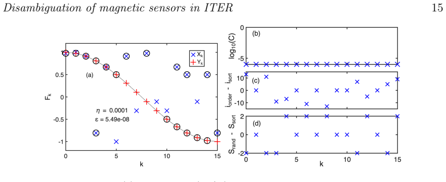
By formulating the disambiguation task as a signed assignment problem whose costs are the squared differences between measured signals and Biot-Savart predictions from all active-coil combinations, the Hungarian algorithm recovers the correct coil locations and polarities for a regularly spaced ITER first-wall array down to a signal-to-noise ratio of 50 in roughly two seconds, yielding reconstruction C>0.97; the same procedure applied to multiple second-wall arrays at fixed toroidal angle yields lower initial recovers that rise to C>0.59 once poloidal-field-coil fields are included in the cost.
What carries the argument
The Hungarian algorithm applied to the cost matrix of squared differences between observed sensor signals and Biot-Savart fields computed for every signed coil assignment.
If this is right
- Commissioning of the magnetic diagnostic set can be completed without scheduling up to 48 dedicated plasma-less discharges.
- The O(N^3) scaling permits the procedure to finish in seconds for arrays of several hundred sensors.
- Including poloidal-field-coil contributions in the cost function measurably improves for second-wall poloidal-flux arrays.
- The same optimisation structure can be applied to other toroidal devices that possess regularly spaced magnetic-sensor arrays.
Where Pith is reading between the lines
- The method could be validated first on existing medium-sized tokamaks whose sensor layouts already contain known wiring errors.
- If field-pattern distinguishability holds at lower signal-to-noise ratios than 50, the same algorithm might tolerate even noisier environments or smaller excitation currents.
- Extending the cost function to include time-varying waveforms rather than steady-state fields could further reduce the number of required energisations.
Load-bearing premise
Different combinations of active coils must produce field patterns at the sensors that remain distinguishable from one another even when measurement noise reaches a signal-to-noise ratio of 50.
What would settle it
Running the algorithm on real ITER commissioning data and finding that the lowest-cost assignment changes or drops below C=0.97 when the same coil set is energised twice under identical conditions would falsify uniqueness at the claimed noise level.
Figures


read the original abstract
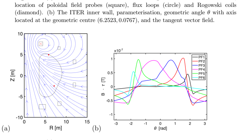
ITER will possess approximately 500 magnetic sensors (mainly measuring poloidal flux) distributed across the first wall. The coils are at known locations but the matching signals not necessarily known. There may also be mistakes in the wiring of the coil polarity. The existing strategy to disambiguate coils uses combinatoric programming of poloidal field coil waveforms of up to 48 discharges of plasma-less operation. An alternate strategy explored in this work is the energisation of a combination of both poloidal and toroidally asymmetric active coils, and Biot-Savart computation of the field solution from all active coils at the sensor coils. A direct brute force permutation of all $N$ coil combinations scales as $O(2^N N!) $ which is intractable for $N>10$. The mathematically formulated optimisation problem was analysed using AI-assisted coding tools, which identified the problem structure as a signed assignment problem and suggested a Hungarian-algorithm-based optimisation strategy, which scales as $O(N^3)$. This search algorithm, when embedded into the magnetic-diagnostic identification problem, was able to disambiguate randomly connected and polarised coils in a regularly spaced array in the ITER first wall (where the the coils are located) down to a signal-to-noise ratio of 50. The computation took 2 seconds. Reconstruction of the actual coil positions in the ITER first wall was achieved high confidence, $C>0.97$. Reconstruction of the second wall poloidal flux coils, which comprised multiple arrays at near constant $\phi$ (each of which is regularly spaced in $\theta$) had a much lower confidence, of $C > 0.15$. By adding the active poloidal field coils to the combined cost function, the confidence increased to $C > 0.59$. This provides the opportunity to reduce the commissioning time of ITER, and is a strategy that could be tested on other toroidal magnetic confinement devices.
Editorial analysis
A structured set of objections, weighed in public.
Referee Report
Summary. The manuscript proposes an alternate strategy for disambiguating ~500 magnetic sensors (primarily poloidal flux) in the ITER first wall, where coil locations are known but connections and polarities may not be. The approach energizes combinations of poloidal and toroidally asymmetric active coils, computes Biot-Savart fields at sensor locations, and solves the resulting signed assignment problem via a Hungarian-algorithm optimization (O(N^3) scaling) rather than brute-force permutation (O(2^N N!)). Simulations on regularly spaced arrays in the ITER first wall achieve disambiguation with confidence C>0.97 down to SNR=50 in ~2 seconds; performance on second-wall coils (multiple arrays at near-constant φ) starts at C>0.15 but rises to C>0.59 when active poloidal-field coils are added to the cost function. The method is positioned as a way to reduce commissioning time relative to the existing 48-discharge combinatoric approach.
Significance. If the simulation results hold under realistic conditions, the work offers a practical, scalable route to sensor disambiguation that could shorten ITER commissioning. The explicit use of AI-assisted coding to recognize the signed-assignment structure and the direct test of the distinguishability assumption on modeled ITER geometry are strengths. The reported performance on regular arrays (C>0.97 at SNR=50) and the quantitative improvement from including poloidal-field coils provide concrete, falsifiable benchmarks.
major comments (2)
- [Abstract] Abstract: the central performance claim (disambiguation to SNR=50 with C>0.97 on regularly spaced arrays) is load-bearing, yet the abstract supplies no information on the precise form of the cost function fed to the Hungarian algorithm or on how additive noise was generated and scaled; without these, the robustness of the reported confidence values cannot be assessed from the given description.
- [Results (second-wall section)] Results on second-wall coils: the drop to C>0.15 (and recovery to C>0.59 when poloidal-field coils are added) is presented as a key finding, but the manuscript does not quantify the degree of pattern degeneracy or provide the explicit combined cost-function expression; this omission directly affects whether the improvement is a general feature of the method or specific to the chosen array geometry.
minor comments (2)
- [Abstract] Abstract contains two typographical errors: 'where the the coils are located' and the missing preposition in 'was achieved high confidence, C>0.97'.
- [Method] The manuscript should include at least one explicit equation for the cost function (or a reference to its definition) so that readers can reproduce the assignment problem exactly.
Simulated Author's Rebuttal
We thank the referee for the constructive comments and the recommendation for minor revision. We address each major comment below and will revise the manuscript accordingly to improve clarity and completeness.
read point-by-point responses
-
Referee: [Abstract] Abstract: the central performance claim (disambiguation to SNR=50 with C>0.97 on regularly spaced arrays) is load-bearing, yet the abstract supplies no information on the precise form of the cost function fed to the Hungarian algorithm or on how additive noise was generated and scaled; without these, the robustness of the reported confidence values cannot be assessed from the given description.
Authors: We agree that the abstract should include these details for transparency. The cost function is the sum of squared residuals between the observed sensor signals and the Biot-Savart predictions (with sign flips allowed for polarity errors). Additive noise is zero-mean Gaussian, scaled to the target SNR relative to the peak signal amplitude. In the revised manuscript we will insert a concise description of both into the abstract. revision: yes
-
Referee: [Results (second-wall section)] Results on second-wall coils: the drop to C>0.15 (and recovery to C>0.59 when poloidal-field coils are added) is presented as a key finding, but the manuscript does not quantify the degree of pattern degeneracy or provide the explicit combined cost-function expression; this omission directly affects whether the improvement is a general feature of the method or specific to the chosen array geometry.
Authors: We accept that explicit quantification and the combined cost-function expression are needed. The combined cost is a weighted sum of the individual assignment costs from the first-wall array and the poloidal-field-coil measurements. Pattern degeneracy arises from the near-constant toroidal angle of the second-wall arrays; we will add the explicit expression and a quantitative measure (e.g., the fraction of permutations within 5 % of the minimum cost) to the revised Results section. revision: yes
Circularity Check
No significant circularity
full rationale
The paper presents a computational method that formulates coil disambiguation as a signed assignment problem solved via the Hungarian algorithm, with forward fields generated from an external Biot-Savart model of known coil positions. Performance metrics (C>0.97 at SNR=50) are obtained by direct simulation on the modeled geometry with injected noise; no parameters are fitted to data and then re-predicted, no uniqueness is imported via self-citation, and no ansatz or renaming reduces the central claim to its inputs by construction. The derivation chain is therefore self-contained against the stated forward model.
Axiom & Free-Parameter Ledger
axioms (1)
- domain assumption Biot-Savart computation from known active-coil currents accurately predicts the field at each sensor location
Reference graph
Works this paper leans on
-
[1]
V D Pustovitov. “Magnetic diagnostics: General principles and the problem of reconstruction of plasma current and pressure profiles in toroidal systems”. In: Nucl. Fusion41 (2001), pp. 721–730.doi:10.1088/0029-5515/41/6/307
-
[2]
I. H. Hutchinson.Principles of Plasma Diagnostics. Cambridge University Press, July 2002.isbn: 9780521803892.doi:10.1017/CBO9780511613630
-
[3]
Fast magnetic fluctuation diagnostics for Alfv´ en eigenmode and magnetohydrodynamics studies at the Joint European Torus
R. F. Heeter et al. “Fast magnetic fluctuation diagnostics for Alfv´ en eigenmode and magnetohydrodynamics studies at the Joint European Torus”. In:Review of Scientific Instruments71.11 (2000), pp. 4092–4106.issn: 00346748.doi:10. 1063/1.1313797
2000
-
[4]
Calibration of the high-frequency magnetic fluctuation diagnostic in plasma devices
L. C. Appel and M. J. Hole. “Calibration of the high-frequency magnetic fluctuation diagnostic in plasma devices”. In:Review of Scientific Instruments 76.9 (Sept. 2005).issn: 00346748.doi:10.1063/1.2009107
-
[5]
Effective Area Measurements of Magnetic Pick-Up Coil Sensors for RFX-mod2
Domenico Abate and Roberto Cavazzana. “Effective Area Measurements of Magnetic Pick-Up Coil Sensors for RFX-mod2”. In:Sensors22.24 (Dec. 2022). issn: 14248220.doi:10.3390/s22249767. REFERENCES24
-
[6]
Magnetic measurements on the TCV Tokamak
J. M. Moret et al. “Magnetic measurements on the TCV Tokamak”. In:Review of Scientific Instruments69.6 (1998), pp. 2333–2348.issn: 00346748.doi:10.1063/ 1.1148940
1998
-
[7]
L. L. Lao et al. “Reconstruction of current profile parameters and plasma shapes in tokamaks”. In:Nucl. Fusion25 (1985), pp. 1611–1622.doi:10.1088/0029- 5515/25/11/007
-
[8]
MHD equilibrium reconstruction in the DIII-D tokamak
L. L. Lao et al. “MHD equilibrium reconstruction in the DIII-D tokamak”. In: Fusion Science and Technology48.2 (2005), pp. 968–977.issn: 15361055.doi: 10.13182/FST48-968
-
[9]
Neto.ITER Commissioning Document: 55.A0 - Magnetics Electronics and Software Technical Basis
A. Neto.ITER Commissioning Document: 55.A0 - Magnetics Electronics and Software Technical Basis. Tech. rep. Feb. 2024
2024
-
[10]
The Hungarian method for the assignment problem,
H. W. Kuhn. “The Hungarian method for the assignment problem”. In:Naval Research Logistics Quarterly2.1-2 (Mar. 1955), pp. 83–97.issn: 0028-1441.doi: 10.1002/nav.3800020109
-
[11]
Fourier decomposition of magnetic perturbations in toroidal plasmas using singular value decomposition
M J Hole and L C Appel. “Fourier decomposition of magnetic perturbations in toroidal plasmas using singular value decomposition”. In:Plasma Physics and Controlled Fusion49.12 (Dec. 2007), pp. 1971–1988.issn: 0741-3335.doi:10. 1088/0741-3335/49/12/002
2007
-
[12]
A high resolution Mirnov array for the mega ampere spherical tokamak
M. J. Hole, L. C. Appel, and R. Martin. “A high resolution Mirnov array for the mega ampere spherical tokamak”. In:Review of Scientific Instruments80.12 (2009).issn: 00346748.doi:10.1063/1.3272713
-
[13]
Qu´ eval.BSmag Toolbox for Matlab
L. Qu´ eval.BSmag Toolbox for Matlab. D¨ usseldorf, 2015
2015
-
[14]
Kay.Fundamentals of statistical signal processing : volume 1 Estimation Theory
Steven M.. Kay.Fundamentals of statistical signal processing : volume 1 Estimation Theory. Prentice-Hall PTR, 1993.isbn: 0133457117. REFERENCES25
1993
-
[15]
Bishop.Pattern recognition and machine learning
Christopher M. Bishop.Pattern recognition and machine learning. Springer Science + Business Media, 2009, p. 738.isbn: 0387310738.doi:10 . 1117 / 1 . 2819119
2009
-
[16]
G. T. Von Nessi and M. J. Hole. “Recent developments in Bayesian inference of tokamak plasma equilibria and high-dimensional stochastic quadratures”. In: Plasma Physics and Controlled Fusion56.11 (Nov. 2014), p. 114011.issn: 13616587.doi:10.1088/0741-3335/56/11/114011
-
[17]
Society for Industrial and Applied Mathematics, 2005, p
Albert Tarantola.Inverse problem theory and methods for model parameter estimation. Society for Industrial and Applied Mathematics, 2005, p. 342.isbn: 0898715725
2005
discussion (0)
Sign in with ORCID, Apple, or X to comment. Anyone can read and Pith papers without signing in.