Non-linear control variate in {δ}f particle-in-cell methods using symplectic neural networks
Pith reviewed 2026-06-30 02:53 UTC · model grok-4.3
The pith
Symplectic neural networks approximate the backward flow to evolve the bulk density as a non-linear control variate in δf PIC methods for plasma simulations.
A machine-rendered reading of the paper's core claim, the machinery that carries it, and where it could break.
Core claim
The paper claims that SympNets can be trained on particle trajectories to serve as an approximation of the backward flow, allowing the bulk density to be evolved as a control variate in the δf PIC method for the Vlasov-Poisson system, with a periodic architecture encoding the periodicity.
What carries the argument
SympNets as approximation of the backward flow, trained using particle trajectories, with periodic variant encoding spatial periodicity.
If this is right
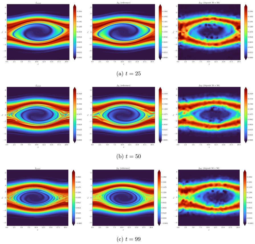
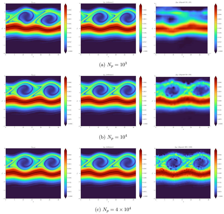
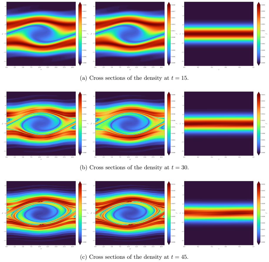
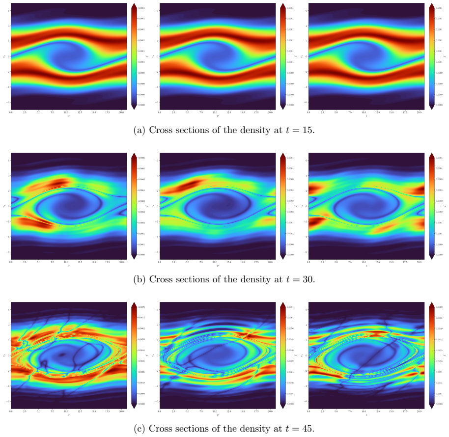
- The approach is validated with numerical results in 1D1V and 3D3V for the Vlasov-Poisson system.
- The periodic SympNet encodes the spatial periodicity into the network.
- The control variate reduces variance without introducing new errors if the approximation is accurate.
Where Pith is reading between the lines
- If the SympNets accurately capture the flow, this method could extend to other kinetic systems beyond Vlasov-Poisson.
- The training on trajectories might allow adaptive control variates that follow non-linear plasma dynamics better than traditional methods.
- Longer simulations could benefit from reduced noise accumulation over time.
Load-bearing premise
SympNets trained on particle trajectories can accurately approximate the backward flow and the periodic variant sufficiently encodes spatial periodicity so that the control variate reduces variance without new errors.
What would settle it
Numerical experiments where the variance in the δf PIC method does not decrease or errors increase when using the SympNet-evolved control variate compared to standard methods.
Figures


read the original abstract
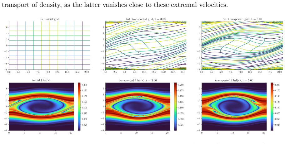
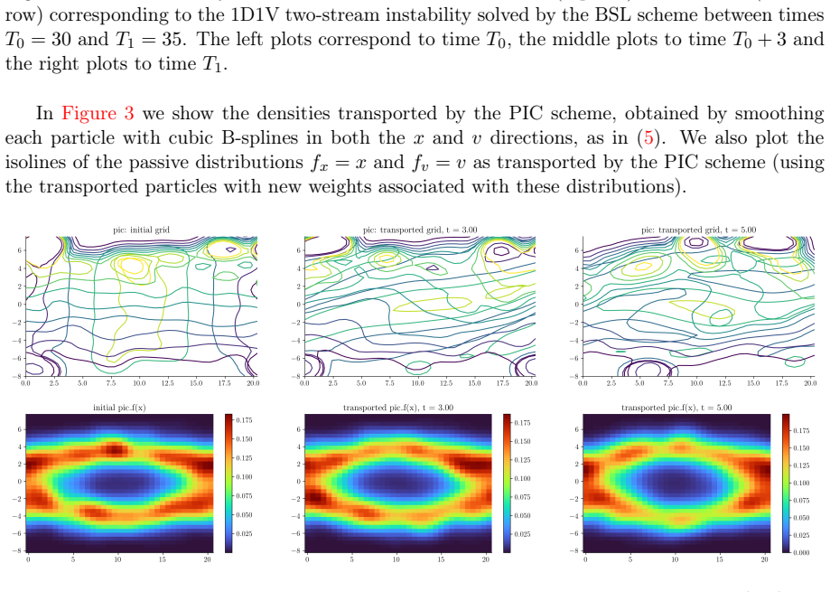
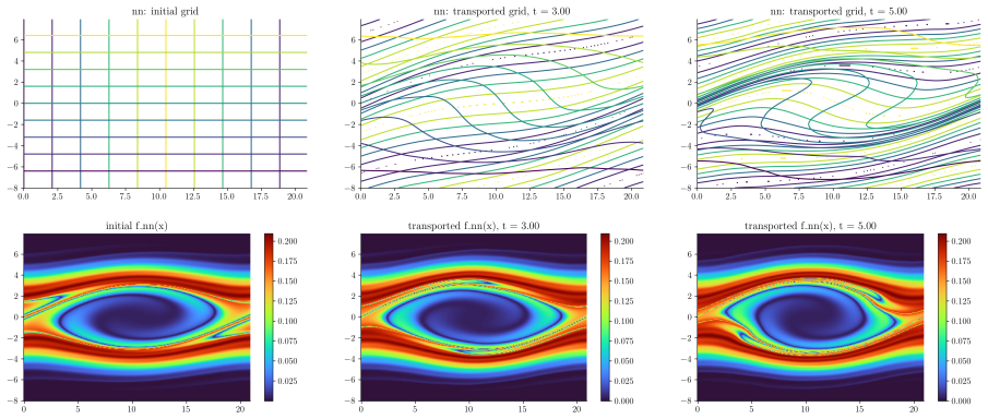
We present a novel {\delta}f particle-in-cell (PIC) method for the kinetic simulation of electrostatic plasmas in which the bulk density, acting as a control variate, is evolved using symplectic neural networks (SympNets). The SympNets are used as an approximation of the backward flow and trained using the particle trajectories. We introduce a periodic variant of the SympNet architecture that encodes the spatial periodicity of the problem into the network itself. We validate the approach with numerical results in 1D1V and 3D3V for the Vlasov-Poisson system.
Editorial analysis
A structured set of objections, weighed in public.
Referee Report
Summary. The paper presents a novel δf particle-in-cell method for electrostatic plasmas in which the bulk density control variate is evolved via symplectic neural networks (SympNets) that approximate the backward flow and are trained on particle trajectories. A periodic variant of the SympNet architecture is introduced to encode spatial periodicity. The approach is validated numerically for the Vlasov-Poisson system in 1D1V and 3D3V.
Significance. If the SympNet approximation to the backward flow is sufficiently accurate and unbiased over long times, the method could enable effective non-linear control variates in δf PIC simulations while preserving symplecticity, offering a route to variance reduction beyond linear control variates in kinetic plasma modeling.
major comments (3)
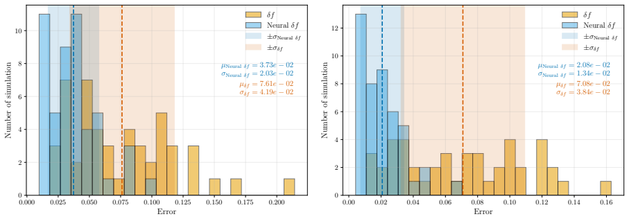
- [Numerical results (1D1V and 3D3V cases)] The validation sections provide no quantitative bounds on the flow approximation error (e.g., trajectory error norms or comparison to exact integrators), no demonstration that the learned control variate remains unbiased over long integration times, and no ablation against standard δf or linear control-variate baselines; this leaves the central variance-reduction claim unsupported.
- [§3 (periodic variant definition)] It is not shown that the periodic SympNet variant preserves the symplectic property of the underlying flow map or that the periodicity encoding does not introduce systematic bias into the weight equation; any such discrepancy would add uncontrolled error to the δf estimator.
- [Method description and training details] The training procedure on particle trajectories is described at a high level but lacks analysis of how approximation errors propagate into the control-variate correction term or whether the method remains consistent as the number of particles increases.
minor comments (2)
- [Throughout] Notation for the weight equation and the SympNet input/output dimensions should be made fully consistent between the method section and the numerical results.
- [Figures] Figure captions for the 1D1V and 3D3V results should explicitly state the number of particles, time steps, and any error metrics shown.
Simulated Author's Rebuttal
We thank the referee for the constructive feedback on our manuscript. We agree that the current version requires additional quantitative support for the central claims and will incorporate the suggested analyses and demonstrations in a revised version. Below we respond point-by-point to the major comments.
read point-by-point responses
-
Referee: [Numerical results (1D1V and 3D3V cases)] The validation sections provide no quantitative bounds on the flow approximation error (e.g., trajectory error norms or comparison to exact integrators), no demonstration that the learned control variate remains unbiased over long integration times, and no ablation against standard δf or linear control-variate baselines; this leaves the central variance-reduction claim unsupported.
Authors: We agree that the presented numerical results lack explicit quantitative bounds on approximation error, long-time unbiasedness checks, and direct ablations. In the revision we will add: (i) trajectory error norms (L2 and max-norm) against a high-order symplectic integrator for the 1D1V test cases; (ii) time-series monitoring of the sample mean of the weights to confirm unbiasedness over extended integration intervals; and (iii) variance-reduction comparisons against both standard δf and linear control-variate baselines, reporting relative variance ratios as functions of time and particle number. revision: yes
-
Referee: [§3 (periodic variant definition)] It is not shown that the periodic SympNet variant preserves the symplectic property of the underlying flow map or that the periodicity encoding does not introduce systematic bias into the weight equation; any such discrepancy would add uncontrolled error to the δf estimator.
Authors: We acknowledge that symplectic preservation for the periodic SympNet and absence of bias in the weight update are not rigorously established in the current text. The revision will include: (i) a short proof that the periodic extension (via appropriate wrapping of the input coordinates) inherits the symplectic property of the base SympNet layers, and (ii) a numerical check that the discrete weight equation remains unbiased when the periodic network is substituted for the exact flow map. revision: yes
-
Referee: [Method description and training details] The training procedure on particle trajectories is described at a high level but lacks analysis of how approximation errors propagate into the control-variate correction term or whether the method remains consistent as the number of particles increases.
Authors: The training description is indeed high-level. We will expand §2 and §4 with: (i) a first-order error-propagation analysis showing how the SympNet residual enters the δf weight correction, and (ii) additional convergence plots demonstrating that the variance-reduction factor remains stable or improves as the particle count is increased from 10^4 to 10^6 while keeping the network architecture fixed. revision: yes
Circularity Check
No circularity; method and validation are independent of fitted inputs
full rationale
The paper proposes a δf PIC scheme in which SympNets approximate the backward flow and are trained on particle trajectories, with a periodic architecture variant introduced to encode periodicity. The central claim is that this yields an effective nonlinear control variate for variance reduction. No equation or derivation in the abstract reduces a reported prediction or result to the training data by construction; the approximation quality is presented as an empirical property verified by separate numerical experiments in 1D1V and 3D3V. No self-citation chain, uniqueness theorem, or ansatz smuggling is invoked to justify the architecture or the control-variate benefit. The load-bearing assumption (accuracy of the learned flow) is therefore an external, falsifiable claim rather than a definitional identity.
Axiom & Free-Parameter Ledger
free parameters (1)
- SympNet weights and biases
invented entities (1)
-
periodic variant of SympNet architecture
no independent evidence
Reference graph
Works this paper leans on
-
[1]
S. J. Allfrey and R. Hatzky. A revisedδ falgorithm for nonlinear PIC simulation.Comput. Phys. Commun., 154(2):98–104, 2003
2003
-
[2]
Amari and S
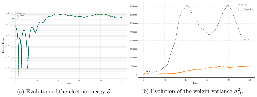
S.-I. Amari and S. C. Douglas. Why natural gradient? InProceedings of the 1998 IEEE International Conference on Acoustics, Speech and Signal Processing, ICASSP’98 (Cat. No. 98CH36181), volume 2, pages 1213–1216. IEEE, 1998. 32 0 10 20 30 40 50 Time t 10−2 10−1 100 101 102 103 Electric Energy Eneural δf Eδf (PIC) ESL (a) Evolution of the electric energyE. ...
1998
-
[3]
T. D. Arber and R. G. L. Vann. A Critical Comparison of Eulerian-Grid-Based Vlasov Solvers.J. Comput. Phys., 180(1):339–357, 2002
2002
-
[4]
A. Y. Aydemir. A unified Monte Carlo interpretation of particle simulations and applications to non-neutral plasmas.Phys. Plasmas, 1(4):822–831, 1994
1994
-
[5]
M. Bachmayr, A. Cohen, A. Kunoth, and O. Mula. Computation and Learning in High Dimensions.Oberwolfach Reports, 22(3):2013–2064, Feb. 2026. ISSN 1660-8933. doi: 10. 4171/owr/2025/37. URLhttps://ems.press/journals/owr/articles/14299515
-
[6]
Beltran-Pulido, I
A. Beltran-Pulido, I. Bilionis, and D. Aliprantis. Physics-Informed Neural Networks for Solving Parametric Magnetostatic Problems.IEEE Trans. Energy Convers., 37(4):2678– 2689, 2022
2022
-
[7]
Bengio, J
Y. Bengio, J. Louradour, R. Collobert, and J. Weston. Curriculum learning. InProceedings of the 26th annual international conference on machine learning, pages 41–48, 2009
2009
-
[8]
Biesek and P
V. Biesek and P. H. de Almeida Konzen. Burgers’ PINNs with implicit Euler Transfer Learning.Rev. Mundi Eng., Tecnol. Gest., 9(4), 2024
2024
-
[9]
C. K. Birdsall and A. B. Langdon.Plasma Physics via Computer Simulation. IOP Publish- ing, 1991
1991
-
[10]
Bottino and E
A. Bottino and E. Sonnendrücker. Monte Carlo particle-in-cell methods for the simulation of the Vlasov–Maxwell gyrokinetic equations.J. Plasma Phys., 81(5), 2015
2015
-
[11]
Bruna, B
J. Bruna, B. Peherstorfer, and E. Vanden-Eijnden. Neural Galerkin schemes with active learning for high-dimensional evolution equations.J. Comput. Phys., 496:112588, 2024
2024
-
[12]
Brunner, E
S. Brunner, E. Valeo, and J. A. Krommes. Collisional delta-fscheme with evolving back- ground for transport time scale simulations.Physics of Plasmas, 6(12):4504–4521, 1999
1999
-
[13]
Campos Pinto, M
M. Campos Pinto, M. Pelz, and P.-H. Tournier. Aδ fPIC method with forward–backward Lagrangian reconstructions.Phys. Plasmas, 30(3), 2023
2023
-
[14]
De Ryck and S
T. De Ryck and S. Mishra. Error analysis for physics-informed neural networks (PINNs) approximating Kolmogorov PDEs.Adv. Comput. Math., 48(6), 2022
2022
-
[15]
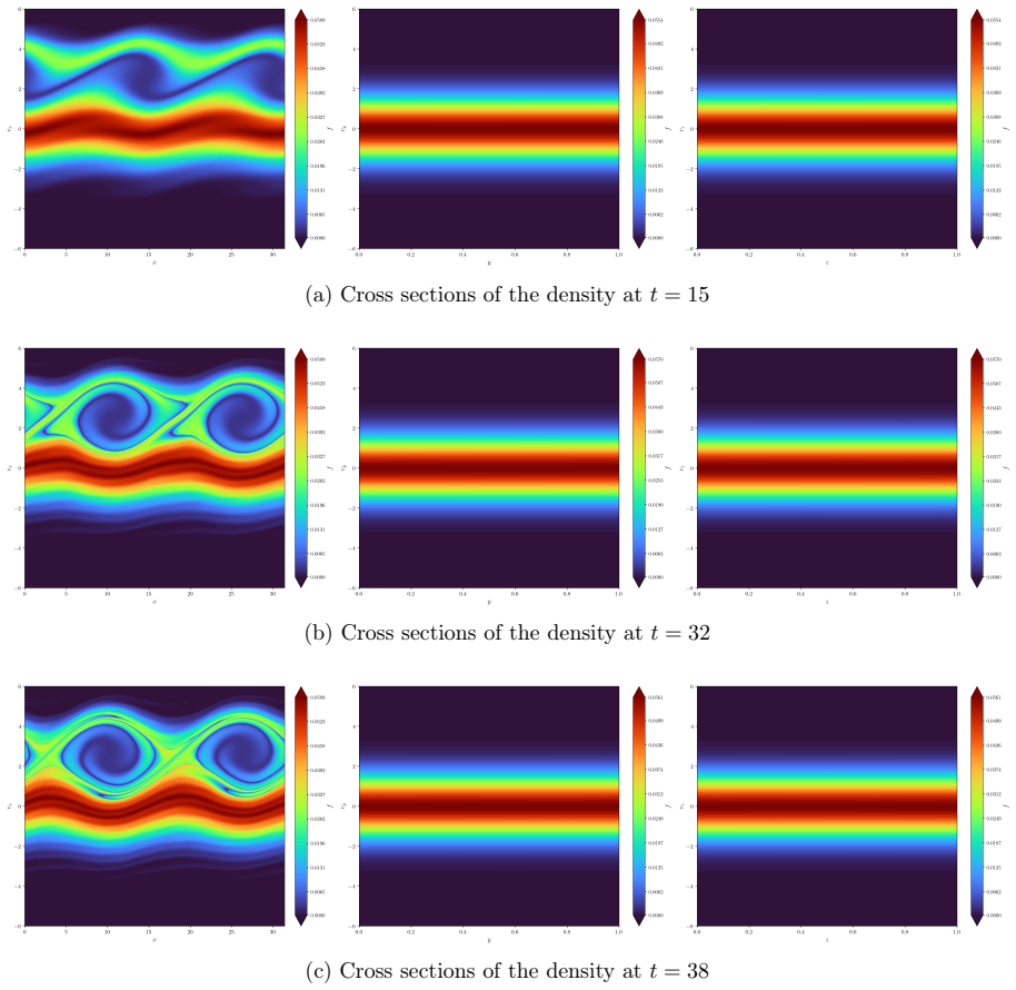
A. M. Dimits and W. W. Lee. Partially Linearized Algorithms in Gyrokinetic Particle Simulation.J. Comput. Phys., 107(2):309–323, 1993. 33 (a) Cross sections of the density att= 15 (b) Cross sections of the density att= 32 (c) Cross sections of the density att= 38 Figure 21: 3D3V bump-on-tail instability from Section 5.2.2: Cross sections of the phase-spac...
1993
-
[16]
Franck, V
E. Franck, V. Michel-Dansac, L. Navoret, and V. Vigon. Neural semi-Lagrangian method for high-dimensional advection-diffusion problems.Comput. Methods Appl. Mech. Engrg., 448(B):118481, 2026
2026
-
[17]
Garbet, Y
X. Garbet, Y. Idomura, L. Villard, and T. H. Watanabe. Gyrokinetic simulations of turbu- lent transport.Nucl. Fusion, 50(4):043002, 2010
2010
-
[18]
Hatzky, R
R. Hatzky, R. Kleiber, A. Könies, A. Mishchenko, M. Borchardt, A. Bottino, and E. Son- nendrücker. Reduction of the statistical error in electromagnetic gyrokinetic particle- in-cell simulations.Journal of Plasma Physics, 85(1):905850112, 2019. doi: 10.1017/ s0022377819000096
2019
-
[19]
Hu and J
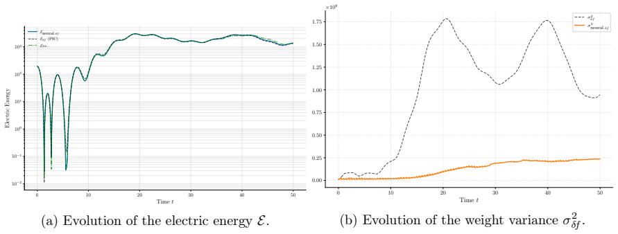
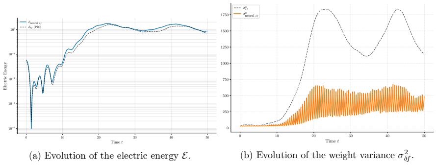
G. Hu and J. A. Krommes. Generalized weighting scheme forδ fparticle-simulation method. Phys. Plasmas, 1(4):863–874, 1994. 34 0 10 20 30 40 50 Time t 10−4 10−3 10−2 10−1 100 Electric Energy Eneural δf Eδf (PIC) (a) Evolution of the electric energyE. 0 10 20 30 40 50 Time t 0 250 500 750 1000 1250 1500 1750 σ2 δf σ2 neural δf (b) Evolution of the weight va...
1994
-
[20]
Tacklingthecurseofdimensionality with physics-informed neural networks.Neural Netw., 176:106369, 2024
Z.Hu, K.Shukla, G.E.Karniadakis, andK.Kawaguchi. Tacklingthecurseofdimensionality with physics-informed neural networks.Neural Netw., 176:106369, 2024
2024
-
[21]
P. Jin, Z. Zhang, A. Zhu, Y. Tang, and G. E. Karniadakis. SympNets: Intrinsic structure- preserving symplectic networks for identifying Hamiltonian systems.Neural Netw., 132: 166–179, 2020
2020
-
[22]
D. P. Kingma and J. Ba. Adam: A method for stochastic optimization. InProceedings of the 3rd International Conference on Learning Representations (ICLR 2015), San Diego, CA, USA, 2015
2015
-
[23]
Kotschenreuther, P
M. Kotschenreuther, P. M. Valanju, S. M. Mahajan, and J. C. Wiley. On heat loading, novel divertors, and fusion reactors.Phys. Plasmas, 14(7), 2007
2007
-
[24]
Krah, X.-Y
P. Krah, X.-Y. Yin, J. Bergmann, J.-C. Nave, and K. Schneider. A characteristic map- ping method for Vlasov–Poisson with extreme resolution properties.Communications in Computational Physics, 35(4):905–937, 2024
2024
-
[25]
S. Ku, R. Hager, C. S. Chang, J. M. Kwon, and S. E. Parker. A new hybrid-Lagrangian numerical scheme for gyrokinetic simulation of tokamak edge plasma.J. Comput. Phys., 315:467–475, 2016
2016
-
[26]
Lanti, N
E. Lanti, N. Ohana, N. Tronko, et al. Orb5: A global electromagnetic gyrokinetic code using the PIC approach in toroidal geometry.Comput. Phys. Commun., 251:107072, 2020
2020
-
[27]
Mildenhall, P
B. Mildenhall, P. P. Srinivasan, M. Tancik, J. T. Barron, R. Ramamoorthi, and R. Ng. NeRF: representing scenes as neural radiance fields for view synthesis.Commun. ACM, 65 (1):99–106, 2021
2021
-
[28]
Müller and M
J. Müller and M. Zeinhofer. Achieving High Accuracy with PINNs via Energy Natural Gradient Descent. In A. Krause, E. Brunskill, K. Cho, B. Engelhardt, S. Sabato, and J. Scarlett, editors,Proceedings of the 40th International Conference on Machine Learning, volume 202 ofProceedings of Machine Learning Research, pages 25471–25485. PMLR, 2023
2023
-
[29]
Murugappan, L
M. Murugappan, L. Villard, S. Brunner, B. F. McMillan, and A. Bottino. Gyrokinetic simulations of turbulence and zonal flows driven by steep profile gradients using a delta-f approach with an evolving background Maxwellian.Phys. Plasmas, 29(10), 2022. 35
2022
-
[30]
Murugappan, L
M. Murugappan, L. Villard, S. Brunner, G. Di Giannatale, B. F. McMillan, and A. Bottino. Gyrokinetic flux-driven simulations in mixed TEM/ITG regime using a delta-f PIC scheme with evolving background.Phys. Plasmas, 31(11), 2024
2024
-
[31]
S. E. Parker and W. W. Lee. A fully nonlinear characteristic method for gyrokinetic simu- lation.Phys. Fluids B, 5(1):77–86, 1993
1993
-
[32]
S. E. Parker, H. E. Mynick, M. Artun, J. C. Cummings, V. Decyk, J. V. Kepner, W. W. Lee, and W. M. Tang. Radially global gyrokinetic simulation studies of transport barriers. Phys. Plasmas, 3(5):1959–1966, 1996
1959
-
[33]
Raissi, P
M. Raissi, P. Perdikaris, and G. E. Karniadakis. Physics-informed neural networks: A deep learning framework for solving forward and inverse problems involving nonlinear partial differential equations.J. Comput. Phys., 378:686–707, 2019
2019
-
[34]
D. Ray, O. Pinti, and A. A. Oberai.Deep Learning and Computational Physics. Springer Nature Switzerland, Cham, 2024. ISBN 978-3-031-59344-4 978-3-031-59345-1. doi: 10.1007/ 978-3-031-59345-1. URLhttps://link.springer.com/10.1007/978-3-031-59345-1
-
[35]
Schild, M
N. Schild, M. Räth, S. Eibl, K. Hallatschek, and K. Kormann. A performance portable im- plementation of the semi-Lagrangian algorithm in six dimensions.Comput. Phys. Commun., 295:108973, 2024
2024
-
[36]
Sonnendrücker, J
E. Sonnendrücker, J. Roche, P. Bertrand, and A. Ghizzo. The Semi-Lagrangian Method for the Numerical Resolution of the Vlasov Equation.J. Comput. Phys., 149(2):201–220, 1999
1999
-
[37]
Sonnendrücker, A
E. Sonnendrücker, A. Wacher, R. Hatzky, and R. Kleiber. A split control variate scheme for PIC simulations with collisions.J. Comput. Phys., 295:402–419, 2015
2015
-
[38]
Stiasny and S
J. Stiasny and S. Chatzivasileiadis. Physics-informed neural networks for time-domain sim- ulations: Accuracy, computational cost, and flexibility.Electr. Pow. Syst. Res., 224:109748, 2023
2023
-
[39]
X. Wang, Y. Chen, and W. Zhu. A Survey on Curriculum Learning.IEEE Trans. Pattern Anal. Mach. Intell., 44(9):4555–4576, 2021
2021
-
[40]
Zhang, G
B. Zhang, G. Cai, H. Weng, W. Wang, L. Liu, and B. He. Physics-informed neural networks for solving forward and inverse Vlasov-Poisson equation via fully kinetic simulation.Mach. Learn.: Sci. Technol., 4(4):045015, 2023. 36
2023
discussion (0)
Sign in with ORCID, Apple, or X to comment. Anyone can read and Pith papers without signing in.