Generating uniform quantum state ensembles with continuous measurement
Pith reviewed 2026-07-01 05:11 UTC · model grok-4.3
The pith
Homogeneous continuous monitoring generates uniform ensembles of pure and mixed quantum states.
A machine-rendered reading of the paper's core claim, the machinery that carries it, and where it could break.
Core claim
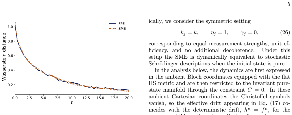
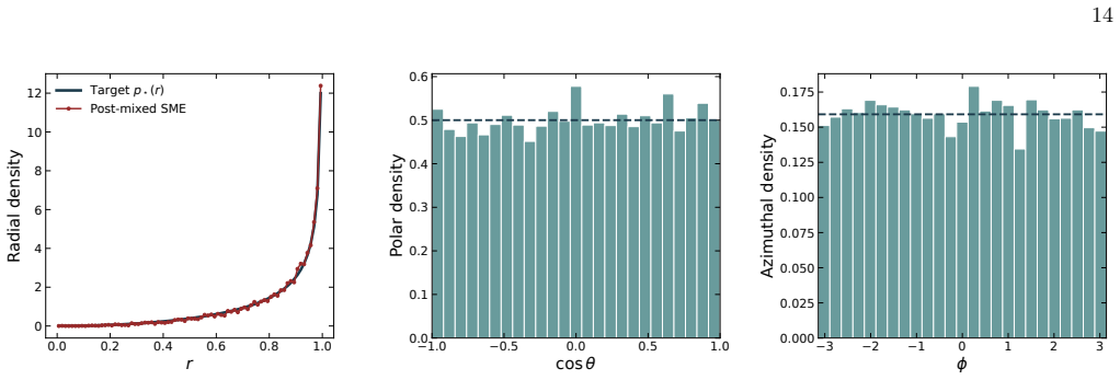
Using the SU(d) Bloch representation, the authors derive the associated Langevin and Fokker-Planck equations and identify geometric conditions under which homogeneous monitoring causes global convergence to the uniform pure-state ensemble. They then extend the analysis to mixed states, showing that homogeneous purity-dependent decoherence rates generate uniform Hilbert-Schmidt and Bures ensembles of qubit states through an effective nonlinear stochastic evolution. They additionally introduce a post-mixing protocol for qubits in which target mixed-state ensembles are assembled by classically sampling trajectories generated with different fixed efficiencies.
What carries the argument
Geometric conditions on the monitoring operators, derived from the SU(d) Bloch representation and Fokker-Planck analysis, that make the uniform distribution the unique stationary solution of the stochastic evolution.
Load-bearing premise
The geometric conditions on the monitoring operators are sufficient to guarantee global convergence without additional assumptions on initial states or higher-order noise terms.
What would settle it
An experiment or simulation in which the long-time distribution of states under homogeneous monitoring satisfying the stated geometric conditions deviates from the uniform pure-state ensemble would falsify the global convergence claim.
Figures


read the original abstract
We investigate the generation of uniform quantum state ensembles via continuous measurement. Using the $SU(d)$ Bloch representation, we derive the associated Langevin and Fokker-Planck equations and identify geometric conditions under which homogeneous monitoring causes global convergence to the uniform pure-state ensemble. We then extend the analysis to mixed states, showing that homogeneous purity-dependent decoherence rates generate uniform Hilbert-Schmidt and Bures ensembles of qubit states through an effective nonlinear stochastic evolution. Additionally, we introduce a post-mixing protocol for qubits: target mixed-state ensembles are assembled by classically sampling trajectories generated with different fixed efficiencies (or decoherence rates). This provides an experimentally feasible route to reconstructing Hilbert-Schmidt and Bures-random mixed-state ensembles, demonstrating that continuous monitoring provides both an exact dynamical generator of Haar-random pure states and a practical route to constructing mixed-state ensembles.
Editorial analysis
A structured set of objections, weighed in public.
Referee Report
Summary. The manuscript claims that continuous measurement with homogeneous monitoring operators satisfying geometric conditions derived from the SU(d) Bloch representation yields global convergence to the uniform (Haar) pure-state ensemble, as shown via associated Langevin and Fokker-Planck equations. For qubit mixed states, purity-dependent decoherence rates are asserted to produce uniform Hilbert-Schmidt and Bures ensembles through an effective nonlinear stochastic process. A post-mixing protocol is proposed in which trajectories at different fixed efficiencies are classically sampled to assemble target mixed-state ensembles, providing an experimentally feasible route to these distributions.
Significance. If the claims hold, the work supplies a dynamical mechanism for generating Haar-random pure states and standard mixed-state ensembles directly from continuous monitoring, which would be useful for quantum state preparation, random benchmarking, and simulation protocols in quantum information. The geometric conditions on monitoring operators give a concrete design criterion, and the post-mixing protocol is practically relevant. The approach correctly employs standard tools (Bloch vectors, Fokker-Planck) to obtain stationarity results, though the extension to global convergence is the key unverified step.
major comments (2)
- [Fokker-Planck analysis] Fokker-Planck analysis (main derivation section): the geometric conditions on monitoring operators are shown to leave the uniform Haar measure invariant, but invariance of the measure does not establish global convergence or uniqueness of the attractor. No Lyapunov function, ergodicity argument, or control of Itô corrections is supplied to rule out other invariant sets or slow mixing on the Bloch manifold.
- [Mixed-state ensembles] Mixed-state section: the nonlinear stochastic evolution with purity-dependent rates is derived and shown to admit the Hilbert-Schmidt and Bures measures as stationary distributions, yet the same gap exists—no argument demonstrates that these are the unique global attractors from arbitrary initial mixed states.
minor comments (3)
- [Abstract] Abstract: the phrasing 'global convergence' should be qualified to match the body, which primarily establishes stationarity under the geometric conditions.
- [Bloch representation] Notation: the mapping from monitoring operators to the drift/diffusion coefficients in the Bloch representation would benefit from an explicit d=2 example to improve readability.
- [References] References: prior literature on continuous-measurement generation of random states and on ergodicity of quantum stochastic processes should be cited for context.
Simulated Author's Rebuttal
We are grateful to the referee for their thorough review and insightful comments, which have helped us identify areas for improvement in our manuscript on generating uniform quantum state ensembles with continuous measurement. We address each major comment below and outline the revisions we will make.
read point-by-point responses
-
Referee: [Fokker-Planck analysis] Fokker-Planck analysis (main derivation section): the geometric conditions on monitoring operators are shown to leave the uniform Haar measure invariant, but invariance of the measure does not establish global convergence or uniqueness of the attractor. No Lyapunov function, ergodicity argument, or control of Itô corrections is supplied to rule out other invariant sets or slow mixing on the Bloch manifold.
Authors: We agree that demonstrating invariance of the Haar measure is not sufficient by itself to prove global convergence. Our geometric conditions ensure stationarity of the uniform distribution, but to establish it as the unique global attractor, we will add to the revised manuscript a Lyapunov function based on the L2 norm of the deviation of the density from uniformity. We will compute its time derivative along the Fokker-Planck flow, showing it is strictly negative except at the uniform measure, thereby ruling out other invariant sets and confirming global convergence. This will also explicitly account for any Itô correction terms in the Bloch representation. revision: yes
-
Referee: [Mixed-state ensembles] Mixed-state section: the nonlinear stochastic evolution with purity-dependent rates is derived and shown to admit the Hilbert-Schmidt and Bures measures as stationary distributions, yet the same gap exists—no argument demonstrates that these are the unique global attractors from arbitrary initial mixed states.
Authors: We concur that the same issue applies to the mixed-state ensembles. While the purity-dependent rates make the target measures stationary, global attraction needs to be proven. In the revision, we will introduce a suitable Lyapunov functional for the nonlinear stochastic process on the Bloch ball, demonstrating convergence to the Hilbert-Schmidt and Bures distributions from any initial mixed state. This will complete the argument for uniqueness of the attractors. revision: yes
Circularity Check
No circularity; derivations from standard stochastic calculus are self-contained
full rationale
The paper starts from the standard SU(d) Bloch representation of the quantum state and derives the associated Langevin and Fokker-Planck equations under continuous monitoring. Geometric conditions on the monitoring operators are identified such that the uniform (Haar) measure is invariant. These steps use established Itô calculus and Fokker-Planck analysis without any reduction of the target ensemble to a fitted parameter, self-defined quantity, or load-bearing self-citation. The post-mixing protocol for mixed-state ensembles is likewise constructed from the same stochastic trajectories without circular renaming or ansatz smuggling. The derivation chain remains independent of its conclusions.
Axiom & Free-Parameter Ledger
axioms (2)
- domain assumption SU(d) Bloch representation is sufficient to capture the dynamics under continuous monitoring
- domain assumption Homogeneous monitoring operators satisfy the geometric conditions needed for convergence
Reference graph
Works this paper leans on
-
[1]
D. N. Page, Average entropy of a subsystem, Phys. Rev. Lett.71, 1291 (1993)
1993
-
[2]
Popescu, A
S. Popescu, A. J. Short, and A. Winter, Entanglement and the foundations of statistical mechanics, Nature Physics2, 754 (2006)
2006
-
[3]
Goldstein, J
S. Goldstein, J. L. Lebowitz, R. Tumulka, and N. Zangh` ı, Canonical typicality, Phys. Rev. Lett.96, 050403 (2006)
2006
-
[4]
M. A. Nielsen and I. L. Chuang,Quantum Computa- tion and Quantum Information: 10th Anniversary Edi- tion(Cambridge University Press, 2010)
2010
-
[5]
Zyczkowski and H.-J
K. Zyczkowski and H.-J. Sommers, Induced measures in the space of mixed quantum states, Journal of Physics A: Mathematical and General34, 7111 (2001)
2001
-
[6]
Bengtsson and K
I. Bengtsson and K. Zyczkowski,Geometry of Quan- tum States: An Introduction to Quantum Entanglement (Cambridge University Press, 2006)
2006
-
[7]
Emerson, Y
J. Emerson, Y. S. Weinstein, M. Saraceno, S. Lloyd, and D. G. Cory, Pseudo-random unitary operators for quan- tum information processing, Science302, 2098 (2003)
2098
-
[8]
Mezzadri, How to generate random matrices from the classical compact groups, Notices of the American Math- 17 ematical Society54, 592 (2007)
F. Mezzadri, How to generate random matrices from the classical compact groups, Notices of the American Math- 17 ematical Society54, 592 (2007)
2007
-
[9]
Collins and I
B. Collins and I. Nechita, Random matrix techniques in quantum information theory, J. Math. Phys.57, 015215 (2015)
2015
-
[10]
W. W. Ho and S. Choi, Exact emergent quantum state designs from quantum chaotic dynamics, Phys. Rev. Lett. 128, 060601 (2022)
2022
-
[11]
J. Choi, A. L. Shaw, I. S. Madjarov, X. Xie, R. Finkel- stein, J. P. Covey, J. S. Cotler, D. K. Mark, H.-Y. Huang, A. Kale, H. Pichler, F. G. S. L. Brand˜ ao, S. Choi, and M. Endres, Preparing random states and benchmarking with many-body quantum chaos, Nature613, 468 (2023)
2023
-
[12]
Zhang, P
B. Zhang, P. Xu, X. Chen, and Q. Zhuang, Holographic deep thermalization for secure and efficient quantum ran- dom state generation, Nat. Commun.16, 6341 (2025)
2025
-
[13]
H. J. D. Miller, Covariant currents and a thermodynamic uncertainty relation on curved manifolds, Proceedings of the Royal Society A: Mathematical, Physical and Engi- neering Sciences481, 20240686 (2025)
2025
-
[14]
C. S. Jackson, How to implement the generalized- coherent-state povm via nonadaptive continuous isotropic measurement (2019), arXiv:1903.02045 [quant- ph]
work page internal anchor Pith review Pith/arXiv arXiv 2019
-
[15]
Benoist, M
T. Benoist, M. Fraas, Y. Pautrat, and C. Pellegrini, In- variant measure for stochastic schr¨ odinger equations, An- nales Henri Poincar´ e22, 347 (2021)
2021
-
[16]
X. Liu, J. Zhuang, W. Hou, and Y.-Z. You, Measurement-based quantum diffusion models (2025), arXiv:2508.08799 [quant-ph]
work page internal anchor Pith review Pith/arXiv arXiv 2025
-
[17]
Shojaee, C
E. Shojaee, C. S. Jackson, C. A. Riofr´ ıo, A. Kalev, and I. H. Deutsch, Optimal pure-state qubit tomography via sequential weak measurements, Phys. Rev. Lett.121, 130404 (2018)
2018
-
[18]
Jacobs and D
K. Jacobs and D. A. Steck, A straightforward introduc- tion to continuous quantum measurement, Contempo- rary Physics47, 279 (2006)
2006
-
[19]
Zyczkowski, K
K. Zyczkowski, K. A. Penson, I. Nechita, and B. Collins, Generating random density matrices, Journal of Mathe- matical Physics52, 062201 (2011)
2011
-
[20]
H. M. Wiseman and G. J. Milburn,Quantum Measure- ment and Control(Cambridge University Press, 2009)
2009
-
[21]
Pfeifer,The Lie Algebras su(N): An Introduction (Birkh¨ auser Basel, Basel, 2003)
W. Pfeifer,The Lie Algebras su(N): An Introduction (Birkh¨ auser Basel, Basel, 2003)
2003
-
[22]
Kimura, The bloch vector for n-level systems, Phys
G. Kimura, The bloch vector for n-level systems, Phys. Lett. A314, 339 (2003)
2003
-
[23]
Albarelli and M
F. Albarelli and M. G. Genoni, A pedagogical introduc- tion to continuously monitored quantum systems and measurement-based feedback, Physics Letters A494, 129260 (2024)
2024
-
[24]
C. W. Gardiner,Stochastic Methods: A Handbook for the Natural and Social Sciences, 4th ed., Springer Series in Synergetics (Springer Berlin, Heidelberg, 2009)
2009
-
[25]
Georgi,Lie Algebras In Particle Physics: From Isospin To Unified Theories, 1st ed
H. Georgi,Lie Algebras In Particle Physics: From Isospin To Unified Theories, 1st ed. (CRC Press, 2000)
2000
-
[26]
Graham, Covariant stochastic calculus in the sense of itˆ o, Phys
R. Graham, Covariant stochastic calculus in the sense of itˆ o, Phys. Lett. A109, 209 (1985)
1985
-
[27]
Risken,The Fokker-Planck Equation: Methods of So- lution and Applications, 2nd ed., Springer Series in Syn- ergetics, Vol
H. Risken,The Fokker-Planck Equation: Methods of So- lution and Applications, 2nd ed., Springer Series in Syn- ergetics, Vol. 18 (Springer-Verlag, Berlin, Heidelberg, 1989)
1989
-
[28]
Villani, The wasserstein distances, inOptimal Trans- port: Old and New(Springer Berlin Heidelberg, Berlin, Heidelberg, 2009) pp
C. Villani, The wasserstein distances, inOptimal Trans- port: Old and New(Springer Berlin Heidelberg, Berlin, Heidelberg, 2009) pp. 93–111
2009
-
[29]
Annby-Andersson, F
B. Annby-Andersson, F. Bakhshinezhad, D. Bhat- tacharyya, G. De Sousa, C. Jarzynski, P. Samuelsson, and P. P. Potts, Quantum fokker-planck master equation for continuous feedback control, Phys. Rev. Lett.129, 050401 (2022)
2022
-
[30]
Vijay, C
R. Vijay, C. Macklin, D. H. Slichter, S. J. Weber, K. W. Murch, R. Naik, A. N. Korotkov, and I. Siddiqi, Stabi- lizing rabi oscillations in a superconducting qubit using quantum feedback, Nature490, 77 (2012)
2012
-
[31]
K. W. Murch, R. Vijay, and I. Siddiqi, Weak measure- ment and feedback in superconducting quantum circuits, inSuperconducting Devices in Quantum Optics, edited by R. H. Hadfield and G. Johansson (Springer Interna- tional Publishing, Cham, 2016) pp. 163–185
2016
-
[32]
Rist` e, C
D. Rist` e, C. C. Bultink, K. W. Lehnert, and L. DiCarlo, Feedback control of a solid-state qubit using high-fidelity projective measurement, Phys. Rev. Lett.109, 240502 (2012)
2012
-
[33]
H. M. Wiseman, Quantum theory of continuous feedback, Phys. Rev. A49, 2133 (1994)
1994
-
[34]
Barchielli and M
A. Barchielli and M. Gregoratti, Quantum measurements in continuous time, non-markovian evolutions and feed- back, Philosophical Transactions of the Royal Society A: Mathematical, Physical and Engineering Sciences370, 5364–5385 (2012)
2012
-
[35]
Guryanova, N
Y. Guryanova, N. Friis, and M. Huber, Ideal projective measurements have infinite resource costs, Quantum4, 222 (2020)
2020
-
[36]
Lecocq, L
F. Lecocq, L. Ranzani, G. A. Peterson, K. Cicak, X. Y. Jin, R. W. Simmonds, J. D. Teufel, and J. Aumentado, Efficient qubit measurement with a nonreciprocal mi- crowave amplifier, Phys. Rev. Lett.126, 020502 (2021)
2021
-
[37]
Eddins, J
A. Eddins, J. M. Kreikebaum, D. M. Toyli, E. M. Levenson-Falk, A. Dove, W. P. Livingston, B. A. Lev- itan, L. C. G. Govia, A. A. Clerk, and I. Siddiqi, High- efficiency measurement of an artificial atom embedded in a parametric amplifier, Phys. Rev. X9, 011004 (2019)
2019
-
[38]
C. L. Lawson and R. J. Hanson,Solving Least Squares Problems, Classics in Applied Mathematics, Vol. 15 (So- ciety for Industrial and Applied Mathematics, Philadel- phia, PA, 1995)
1995
-
[39]
H¨ ubner, Explicit computation of the bures distance for density matrices, Phys
M. H¨ ubner, Explicit computation of the bures distance for density matrices, Phys. Lett. A163, 239 (1992)
1992
-
[40]
I. Layton and H. J. D. Miller, Restoring the second law to classical-quantum dynamics (2025), arXiv:2504.10587 [quant-ph]
-
[41]
McKeever, Continuous measurement simulations for uniform quantum ensembles, 10.48420/32760963 (2026)
T. McKeever, Continuous measurement simulations for uniform quantum ensembles, 10.48420/32760963 (2026)
-
[42]
H. F. Trotter, On the product of semi-groups of opera- tors, Proceedings of the American Mathematical Society 10, 545 (1959)
1959
-
[43]
M. Cuturi, Sinkhorn distances: lightspeed computation of optimal transport, inProceedings of the 27th Interna- tional Conference on Neural Information Processing Sys- tems - Volume 2, NIPS’13 (Curran Associates Inc., Red Hook, NY, USA, 2013) p. 2292–2300. 18 Appendix A: Weak measurements for non-commuting observables In this appendix we briefly justify th...
2013
-
[44]
Projective measurements Consider two observables with spectral decompositions A= X a aPa, B= X b bQb,(A1) where{P a}and{Q b}are orthogonal projectors. The associated nonselective measurement channels are ΦA(ρ) = X a PaρPa,Φ B(ρ) = X b QbρQb.(A2) Composing these maps yields ΦA ◦Φ B(ρ) = X a,b PaQb ρ QbPa,(A3) ΦB ◦Φ A(ρ) = X a,b QbPa ρ PaQb.(A4) These expre...
-
[45]
For a Hermitian observable A, a symmetric weak measurement may therefore be written as K(A) ± = 1√ 2 1±εA− ε2 2 A2 +O(ε 3),(A6) whereε≪1 controls the measurement strength
Weak measurements By contrast, weak measurements are described by Kraus operators close to the identity. For a Hermitian observable A, a symmetric weak measurement may therefore be written as K(A) ± = 1√ 2 1±εA− ε2 2 A2 +O(ε 3),(A6) whereε≪1 controls the measurement strength. The corresponding nonselective channel is EA(ρ) = X ± K(A) ± ρK(A)† ± (A7) =ρ+ε ...
-
[46]
In such a scheme, each observable is measured for a short intervalδt, with the measurement basis cycled sufficiently quickly that no single observable dominates the dynamics [16]
Alternative interpretation Furthermore, simultaneous monitoring of a complete operator basis may be understood, equivalently, as the limit of a rapid sequence of weak measurements performed along different measurement axes. In such a scheme, each observable is measured for a short intervalδt, with the measurement basis cycled sufficiently quickly that no ...
-
[47]
Hamiltonian contribution Using (1), dxl H =−i X j hj Tr ([Sl, Sj]ρ)dt = X j,k hjfljk Tr (Skρ)dt = X j,k hjfljk xkdt.(B5) Relabelling indices and using antisymmetry off ijk gives f l H =h jfljk xk,(B6) as quoted in Eq. (8)
-
[48]
We can also rotate some indices for future simplification, and use repeated indices properties of theSU(d) structure constant,f ijj = 0 valid for alliandj(from (14))
Dissipative contribution For a Hermitian jump operatorL= √ 2λ Sj, D[L]ρ= 2λ SjρSj − 1 2 {S2 j , ρ} .(B7) 20 The full dissipative contribution is therefore obtained by summing over all monitored and unmonitored channels with total rate lj = 2kj + 2γj.(B8) Thus X j D[cj]ρ+ X j D[ξj]ρ= X j lj SjρSj − 1 2 {S2 j , ρ} .(B9) To project this term, we repeatedly u...
-
[49]
Stochastic contribution For the innovation superoperator with Hermitian jump operatorc j = p 2kj Sj, H[cj]ρ= p 2kj (Sjρ+ρS j −2 Tr(Sjρ)ρ).(B16) We find Tr(Sl H[cj]ρ) = X j p 2kj [Tr ({Sl, Sj}ρ)−2x lxj]dW j (B17) = X j p 2kj Tr n 4 d 1dδlj + 2 X m gljmSm o ρ −2x lxj dWj (B18) = p 2kl 4 d dWl + X j,m 2 p 2kj gljmxm dWj − X j 2 p 2kj xlxj dWj (B19) 21 Includ...
-
[50]
Starting from the noise amplitudes σµ j = p 2kjηj 4 d δµj + 2gµjmxm −2x µxj ,(C1) the diffusion tensor isD µν =P j σµ j σν j
Diffusion tensor and derivative identities In this appendix we record the explicit diffusion tensor and the Euclidean derivative identities used in the homoge- neous calculations, under HS geometry. Starting from the noise amplitudes σµ j = p 2kjηj 4 d δµj + 2gµjmxm −2x µxj ,(C1) the diffusion tensor isD µν =P j σµ j σν j . Assuming uncorrelated Wiener in...
-
[51]
We use (14) throughout
Drift vector and derivative identities We provide here some useful expressions for the drift vectorf ν and its derivatives under different conditions. We use (14) throughout. From (8) and (9), the full drift vector can be defined,f l =f l H +f l diss. The Hamiltonian driftf l H does not simplify under homogeneous conditions but,f l diss reduces to f l dis...
-
[52]
Using the divergence theorem onM, Z V ∇µJ µ dV= Z ∂V ⟨J,ˆn⟩dS,(D5) Eq
Continuity equation Probability conservation implies that, for any regionV ⊂ Mwith boundary∂Vand outward unit normal ˆn, the rate of change of probability insideVequals the probability flux across the boundary: d dt Z V ϱ dV=− Z ∂V ⟨J,ˆn⟩dS,(D4) whereJ µ is the probability current. Using the divergence theorem onM, Z V ∇µJ µ dV= Z ∂V ⟨J,ˆn⟩dS,(D5) Eq. (D4...
-
[53]
Applying Itˆ o’s lemma to Eq
Applying Itˆ o’s Lemma To determine the probability current, letκ(⃗ x) be a smooth test function. Applying Itˆ o’s lemma to Eq. (D1) in local coordinates gives dκ=∂ νκ dxν + 1 2 ∂µ∂νκ dxµdxν.(D8) The second partial derivative is not tensorial and therefore cannot appear directly in a coordinate-invariant expression. Since∂ νκis a covector, its covariant d...
-
[54]
For the drift term, Z M hν(∂νκ)ϱ dV= Z M ∇ν(κhνϱ)dV− Z M κ∇ ν(hνϱ)dV =− Z M κ∇ ν(hνϱ)dV,(D17) where the boundary contribution vanishes
Integration by parts Using the covariant divergence theorem over the entire manifoldM, Z M ∇µV µ dV= 0,(D16) for sufficiently regular vector fields satisfying appropriate boundary conditions, we now integrate by parts to move derivatives fromκontoϱ. For the drift term, Z M hν(∂νκ)ϱ dV= Z M ∇ν(κhνϱ)dV− Z M κ∇ ν(hνϱ)dV =− Z M κ∇ ν(hνϱ)dV,(D17) where the bou...
-
[55]
Sinceg abn is symmetric ina, b, 2gabn˜vaxb = 2(d−2) d ˜vn,(E11) and therefore gabn˜vaxb = d−2 d ˜vn,(E12) which is Eq
Tangential derivative identity A further identity used in the proof of condition (iv) is obtained by differentiating gabnxaxb = 2(d−2) d xn (E10) along a tangent direction ˜va. Sinceg abn is symmetric ina, b, 2gabn˜vaxb = 2(d−2) d ˜vn,(E11) and therefore gabn˜vaxb = d−2 d ˜vn,(E12) which is Eq. (52). Appendix F: Wasserstein calculation To quantify converg...
-
[56]
Since the FPE is formulated in Cartesian Bloch coordinates, we express the metric in the same coordinate system
Metric and Christoffel symbols The standard radial form of the Bures metric for a qubit is [6, 39] ds2 = dr2 1−r 2 +r 2dΩ2 (I1) wherer 2 =x 2 +y 2 +z 2 anddΩ 2 =dθ 2 + sin2(θ)dφ 2 withθandφthe usual polar and azimuthal angle respectively. Since the FPE is formulated in Cartesian Bloch coordinates, we express the metric in the same coordinate system. Using...
-
[57]
The covariant divergence of a vector fieldF ν is ∇νF ν =∂ νF ν + Γν νk F k,(I9) where, for the Bures metric, Γ ν νk = xk 1−r2
Covariant derivatives of the drift vector and diffusion tensor The stationarity condition depends on the divergence of the effective drift,h ν =f ν + 1 2Γν ijDij, which we evaluate term by term. The covariant divergence of a vector fieldF ν is ∇νF ν =∂ νF ν + Γν νk F k,(I9) where, for the Bures metric, Γ ν νk = xk 1−r2 . Substituting the homogeneous deter...
-
[58]
ODE forγ(C) Substituting the above expressions into the stationarity condition,∇ νhν − 1 2 ∇ν∇µDµν = 0, and expressingr 2 = 1+ 2C, gives the differential equation forγ B(C) as in Eq. (80). Motivated by the linear dependence of the inhomogeneous term onC, we seek a solution of the formγ B(C) =bC. Substituting this ansatz into the ODE immediately yields Eq....
discussion (0)
Sign in with ORCID, Apple, or X to comment. Anyone can read and Pith papers without signing in.