REVIEW 3 major objections 4 minor 18 references
Cluster-Weighted Training of Deep Surrogate Models for Subgrid Turbulent Transport
T0 review · 3 major / 4 minor · reviewed 2026-07-10 · grok-4.5
Pith's one-line read Cluster-weighted training cuts CNN error on solar Reynolds stresses by 34 percent and raises R^{2} from 0.54 to 0.80.
desk verdict Solid empirical lift from K-Means error reweighting on a solar Reynolds-stress CNN; the 34% MSE / R^{2} gains are real for this setup, but rest on an unablated (T0, α) schedule and still lack closed-loop physics checks. read the letter →
The pith
A machine-rendered reading of the paper's core claim, the machinery that carries it, and where it could break.
The reading
What carries the argument
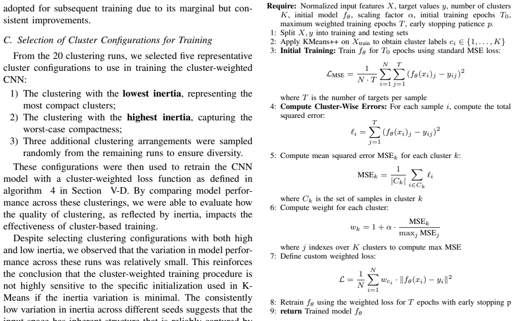
Cluster-weighted loss: after ten epochs of uniform training, samples belonging to each K-Means cluster are multiplied by a scalar proportional to that cluster’s residual MSE; the reweighted network is then fine-tuned to completion.
What would settle it
Retrain the identical CNN architecture on the same solar cubes using a non-cluster importance scheme (for example, uncertainty-based or residual-based sample weights) and check whether the 34 % MSE reduction and the R^{2} jump to 0.80 still appear; if they do not, the clustering step is essential.
Extended reading notes
Core claim
When a 3-D CNN that predicts the six Reynolds-stress components is retrained with a loss reweighted by the mean squared error of five K-Means clusters (weights wk = 1 + 3 · MSEk / max MSEj), average MSE falls from 4.89 × 10^18 to 3.01 × 10^18 and average R^{2} rises from 0.54 to 0.80 relative to the identical architecture trained with ordinary MSE.
Load-bearing premise
That the cluster-wise errors measured after only ten epochs of ordinary training give a stable, non-overfitting signal for how much each sample should be weighted thereafter.
Editorial extensions
If this is right
- Lower-resolution StellarBox runs can replace classical subgrid closures with the cluster-weighted CNN and still recover high-resolution Reynolds-stress statistics.
- Off-diagonal stress components, previously only modestly improved by deep networks, now show large error reductions once high-error clusters are emphasized.
- The same reweighting recipe can be applied to any regression task whose input space contains regions of systematically higher residual.
- Inference cost remains identical to the baseline CNN because only the training loss, not the architecture, is changed.
Reading between the lines
- Because the largest gains concentrate between –1 Mm and the photosphere, the method may be especially useful for near-surface magnetoconvection where gradients are sharpest.
- The modest 15–20 % training overhead suggests the technique could be inserted into other large-eddy-simulation pipelines without redesigning the network.
- If magnetic-field channels were added to the input features, the same cluster-weighting loop might further reduce errors in magnetized turbulence.
Editorial analysis
A structured set of objections, weighed in public.
Referee Report
Summary. The paper introduces cluster-weighted training for a 3D CNN surrogate that predicts the six Reynolds-stress components τ ij from local macroscopic velocities and density, using high-resolution StellarBox quiet-Sun cubes. After a short uniform-MSE warm-up (T0=10 epochs), K-Means (K=5) partitions of the 82-dimensional input features supply permanent sample weights wk=1+α·(MSEk/max MSEj) with α=3; the CNN is then retrained under the weighted loss. Relative to the identical architecture trained with uniform MSE, average MSE falls from 4.89 imes10^18 to 3.01 imes10^18 (≈34 %) and average R² rises from 0.54 to 0.80 (Table II), with clearer PDF tails, tighter error histograms and scatter plots (Figs. 5–7) and localized gains in selected clusters and height ranges (Fig. 8). Limited HAC and physics-baseline comparisons are also shown.
Significance. If the reported gains prove robust, the work supplies a practical, architecture-preserving recipe for improving deep surrogates of anisotropic subgrid transport in solar and stellar convection-zone models. The multi-metric evaluation (RMSE per component, PDFs, height-resolved relative improvement) and the explicit algorithmic description (Fig. 4) are strengths that aid reproducibility. The technique is potentially transferable to other regression problems whose error landscape is spatially heterogeneous, which is a useful methodological contribution beyond the immediate solar-physics application.
major comments (3)
- [Section V-D / Fig. 4] Section V-D and the algorithm of Fig. 4 freeze the cluster weights after only T0=10 epochs of uniform training and employ a single hand-chosen scaling α=3. No ablation of T0 or α, nor a control that reweights by a random or magnitude-matched schedule of the same strength, is reported. Because Table II attributes the 34 % MSE / R² gains specifically to cluster-weighted training, these untested choices are load-bearing; without them it remains possible that any aggressive reweighting of the high-error tail after a short warm-up would produce comparable lifts.
- [Tables I–II] Tables I–II report only point estimates of RMSE, average MSE and R². Despite the authors having already generated 20 K-Means seeds and five representative clusterings, no standard deviations, bootstrap intervals or significance tests accompany the headline numbers. The quantitative claim of a 34 % reduction and an R² jump from 0.54 to 0.80 therefore lacks a statistical foundation.
- [Section VI-A / Table I] Section VI-A and Table I compare HAC-based weighting only on a 2.5 % random subset of the training data (memory-limited) and with a different power-law scheme. The resulting under-performance relative to full-data K-Means cannot be interpreted as a fair head-to-head of clustering methods, yet the text presents it as supporting evidence for the superiority of K-Means.
minor comments (4)
- [Abstract] Abstract and conclusion state “34 % lower MSE” without citing the precise average-MSE values of Table II; a parenthetical reference would improve traceability.
- [Fig. 2] Figure 2a reports cluster-wise MSE in cm⁴ s⁻⁴ while the later tables use cm² s⁻²; units should be harmonized or explicitly converted.
- [Section III] The signed-log transform applied to off-diagonal targets is mentioned only briefly; a short formula or reference would help readers reproduce the preprocessing pipeline.
- [Figs. 5–8] Several figure panels (especially Fig. 7 scatter plots) lack axis labels or color-bar units; adding them would improve readability.
Circularity Check
No significant circularity: cluster-weighted improvement is an empirical reweighting result measured on held-out data, not forced by definition or self-citation chain.
full rationale
The paper's central claim (34% MSE reduction and R^{2} lift from 0.54 to 0.80) is produced by an explicit experimental procedure: unsupervised K-Means on input features only, a short uniform-MSE warm-up (T0=10), freezing of per-cluster mean errors into fixed sample weights wk=1+α·(MSEk/max MSEj) with α=3, then full retraining under the weighted loss, followed by evaluation on a held-out test set (Tables I-II, Figs. 5-8, Algorithm in Fig. 4 / Sec. V-D). None of these steps reduces the reported metrics to an identity or to a fitted parameter by construction; the weights are a heuristic derived from early errors and the final numbers are independent measurements. Self-citations to the authors' prior work [3] supply only the CNN architecture, data pipeline and uniform-loss baseline; they are not load-bearing for the weighting gain itself, which is newly measured here against that baseline and against physics-based models. No uniqueness theorem, ansatz smuggling, or renaming of a known result appears. The procedure is therefore self-contained empirical ML methodology, not circular derivation.
Assumptions & free parameters
free parameters (4)
- number of clusters K =
5
- weight scaling factor α =
3
- initial uniform-training epochs T0 =
10
- Adam learning rate and batch size =
0.001 / 128
assumptions (4)
- domain assumption Reynolds stress is defined by τij = <ui uj> − <ui><uj> averaged over the 4×4×4 sub-cube.
- domain assumption A 3×3×3 neighborhood of velocity components plus central density is a sufficient feature set for predicting the six stress components.
- ad hoc to paper K-Means partitions of the input feature space align with regions of systematically higher prediction error, so that reweighting those partitions improves generalization.
- domain assumption Non-overlapping spatial sampling every third sub-cube and 5-minute temporal cadence yield statistically independent training samples.
Cite this review
Pith. "Pith review of Cluster-Weighted Training of Deep Surrogate Models for Subgrid Turbulent Transport." pith.science (2026). https://pith.science/paper/CMHDCEWS
@misc{pith2026260707925,
  author       = {Pith},
  title        = {Pith review of: Cluster-Weighted Training of Deep Surrogate Models for Subgrid Turbulent Transport},
  year         = {2026},
  howpublished = {\url{https://pith.science/paper/CMHDCEWS}},
  note         = {Machine review of arXiv:2607.07925}
}
read the original abstract
Turbulence in the solar interior and atmosphere plays a crucial role in energy transport, yet modeling its subgrid-scale effects remains a major challenge. This study leverages machine learning (ML) models to predict components of the Reynolds stress tensor using high-resolution StellarBox simulations of the quiet Sun. Previously, we have compared a Multi-Layer Perceptron (MLP) and a 3D Convolutional Neural Network (CNN) against physics-based baselines to achieve a lower Mean Squared Error (MSE) and better generalization across various heights and depths in the solar atmosphere. To enhance learning, in this work, we investigate cluster-weighted training using K-Means and Hierarchical Agglomerative Clustering (HAC). By weighing the loss function based on cluster-specific prediction errors, we direct the model's attention to high-error regions. It significantly improves CNN performance, achieving 34% lower MSE and a significantly higher R2 score indicating that integrating deterministic clustering with ML is a promising technique for modeling subgrid turbulence, in particular, and regression in diverse environments, in general.
Figures


Figures from the paper (5 more)


Reference graph
Works this paper leans on
-
[1]
Reynolds Stress Modeling Using Data Driven Machine Learning Algorithms
J. P. Panda, “Reynolds Stress Modeling Using Data Driven Machine Learning Algorithms,”arXiv e-prints, 2021. [Online]. Available: https://doi.org/10.48550/arXiv.2111.07043
work page Pith review arXiv doi:10.48550/arxiv.2111.07043 2021
-
[2]
Physics-informed machine learning for modeling turbulence in supernovae,
P. I. Karpov, C. Huang, I. Sitdikov, C. L. Fryer, S. Woosley, and G. Pilania, “Physics-informed machine learning for modeling turbulence in supernovae,”The Astrophysical Journal, vol. 940, no. 1, p. 26, 2022. [Online]. Available: https://doi.org/10.3847/1538-4357/ac88cc
-
[3]
R. H. Syeda, D. Kempton, V . Sadykov, I. Kitiashvili, and R. Angryk, “Developing machine learning models of subgrid turbulent transport for quiet sun 3d radiative hydrodynamic simulations,” SSRN Preprint No. 5236395, 2025. [Online]. Available: https://ssrn.com/abstract=5236395
work page 2025
-
[4]
I. N. Kitiashvili, S. Couvidat, and A. Lagg, “Using Realistic MHD Simu- lations for Modeling and Interpretation of Quiet-Sun Observations with the Solar Dynamics Observatory Helioseismic and Magnetic Imager,” The Astrophysical Journal, vol. 808, no. 1, p. 59, Jul. 2015. 2.0 1.5 1.0 0.5 0.0 0.5 1.0 1.5 2.0 log10|Predicted| - log10|Target| 0.00 0.25 0.50 0....
work page 2015
-
[5]
Simulations of Stellar Magnetoconvection using the Radiative MHD Code `StellarBox'
A. A. Wray, K. Bensassi, I. N. Kitiashvili, N. N. Mansour, and A. G. Kosovichev, “Simulations of Stellar Magnetoconvection using the Radiative MHD Code ‘StellarBox’,”arXiv e-prints, p. arXiv:1507.07999, Jul. 2015. [Online]. Available: https://doi.org/10. 48550/arXiv.1507.07999
work page Pith review arXiv 2015
-
[6]
Realistic Simulations of Stellar Radiative MHD,
A. A. Wray, K. Bensassiy, I. N. Kitiashvili, N. N. Mansour, and A. G. Kosovichev, “Realistic Simulations of Stellar Radiative MHD,” inVariability of the Sun and Sun-Like Stars: from Asteroseismology to Space Weather, J. P. Rozelot and E. S. Babayev, Eds., 2018, p. 39. [Online]. Available: https://doi.org/10.1007/978-3-319-77199-1 4
-
[7]
A. Nordlund, “Solar Convection,”Solar Physics, vol. 100, p. 209, Oct. 1985. (a) (b) Fig. 8. Cluster-wise median relative improvement of MSE (a) and relative improvements as a function of height (b) across allτ
work page 1985
-
[8]
Revisiting turbulent properties of solar convection with 3D radiative hydrodynamic modeling
I. N. Kitiashvili and A. A. Wray, “Revisiting turbulent properties of solar convection with 3D radiative hydrodynamic modeling,”arXiv e-prints, p. arXiv:2502.00974, Feb. 2025
work page Pith review arXiv 2025
Show all 18 references
-
[9]
General Circulation Experiments with the Primitive Equations,
J. Smagorinsky, “General Circulation Experiments with the Primitive Equations,”Monthly Weather Review, vol. 91, no. 3, p. 99, Jan. 1963. [Online]. Available: https://doi.org/10.1175/1520-0493(1963)091⟨0099: GCEWTP⟩2.3.CO;2
1963 doi
-
[10]
A dynamic subgrid-scale eddy viscosity model,
M. Germano, U. Piomelli, P. Moin, and W. H. Cabot, “A dynamic subgrid-scale eddy viscosity model,”Physics of Fluids A, vol. 3, no. 7, pp. 1760–1765, Jul. 1991. [Online]. Available: https://doi.org/10.1063/1.857955
1991 doi
-
[11]
Reynolds averaged turbulence modelling using deep neural networks with embedded invariance,
J. Ling, A. Kurzawski, and J. Templeton, “Reynolds averaged turbulence modelling using deep neural networks with embedded invariance,” Journal of Fluid Mechanics, vol. 807, pp. 155–166, 2016. [Online]. Available: https://doi.org/10.1017/jfm.2016.615
2016 doi
-
[12]
Physics-informed neural networks: A deep learning framework for solving forward and inverse problems involving nonlinear partial differential equations,
M. Raissi, P. Perdikaris, and G. E. Karniadakis, “Physics-informed neural networks: A deep learning framework for solving forward and inverse problems involving nonlinear partial differential equations,” Journal of Computational Physics, vol. 378, pp. 686–707, 2019
2019
-
[13]
Nonzero Phase Shifts of Acoustic Waves in the Lower Solar Atmosphere Measured from Realistic Simulations and Their Role in Local Helioseismology,
M. Waidele, J. Zhao, and I. N. Kitiashvili, “Nonzero Phase Shifts of Acoustic Waves in the Lower Solar Atmosphere Measured from Realistic Simulations and Their Role in Local Helioseismology,”The Astrophysical Journal, vol. 949, no. 2, p. 99, Jun. 2023
2023
-
[14]
Scikit-learn: Machine learning in Python,
F. Pedregosa, G. Varoquaux, A. Gramfort, V . Michel, B. Thirion, O. Grisel, M. Blondel, P. Prettenhofer, R. Weiss, V . Dubourg, J. Vanderplas, A. Passos, D. Cournapeau, M. Brucher, M. Perrot, and E. Duchesnay, “Scikit-learn: Machine learning in Python,”Journal of Machine Learn...
2011 doi
-
[15]
Data clustering: 50 years beyond k-means,
A. K. Jain, “Data clustering: 50 years beyond k-means,”Pattern Recog- nition Letters, vol. 31, no. 8, pp. 651–666, 2010
2010
-
[16]
Silhouettes: a graphical aid to the interpretation and validation of cluster analysis,
P. J. Rousseeuw, “Silhouettes: a graphical aid to the interpretation and validation of cluster analysis,”Journal of Computational and Applied Mathematics, vol. 20, pp. 53–65, 1987
1987
-
[17]
k-means++: The advantages of careful seeding,
D. Arthur and S. Vassilvitskii, “k-means++: The advantages of careful seeding,” inProceedings of the eighteenth annual ACM-SIAM sym- posium on Discrete algorithms. Society for Industrial and Applied Mathematics, 2007, pp. 1027–1035
2007
-
[18]
Small-scale Dynamo Simulations: Magnetic Field Am- plification in Exploding Granules and the Role of Deep and Shallow Recirculation,
M. Rempel, “Small-scale Dynamo Simulations: Magnetic Field Am- plification in Exploding Granules and the Role of Deep and Shallow Recirculation,”The Astrophysical Journal, vol. 859, no. 2, p. 161, Jun. 2018
2018
Reviewed July 10, 2026 · model on record in the stance chip above.
Discussion (0). Continue with ORCID to comment.