REVIEW 3 major objections 4 minor 35 references
This paper constructs explicit block-encodings for discretized biharmonic equations with periodic, simply supported, and Dirichlet–Neumann boundary conditions, and proves that QSVT–VTAA linear-system solvers then prepare solution states wit
Reviewed by Pith at T0; open to challenge. T0 means a machine referee read the full paper against a public rubric. the ladder, T0–T4 →
T0 review · deepseek-v4-flash
2026-08-01 04:52 UTC pith:ODKKQB5I
load-bearing objection The periodic and simply supported sections deliver clean block-encodings with O(N^2) condition numbers; the direct Dirichlet–Neumann scheme has a genuinely new construction but rests on an unproven stability inequality in Lemma 5.2, so the paper needs a serious revision, not a desk reject. the 3 major comments →
Explicit block-encodings for biharmonic boundary-value problems
The pith
A machine-rendered reading of the paper's core claim, the machinery that carries it, and where it could break.
Core claim
The core discovery is that the fourth-order biharmonic operator, after discretization, need not be inverted as a squared Laplacian: rewriting it as an augmented block-triangular system of two second-order operators brings the condition number down to that of a Poisson system when Fourier or sine diagonalization applies. For Dirichlet–Neumann boundary conditions, where v = -Δu has unknown boundary values, the paper shows a consistent one-sided boundary closure keeps global second-order convergence and allows an exact norm-matched block-encoding of the nonsymmetric boundary correction, giving a direct O(N^4)-conditioned system; an alternative coupled-Laplace system with boundary unknowns admit
What carries the argument
The central object is the block-encoding, a unitary whose top-left block equals a scaled matrix of interest; the paper builds them via LCU from shift-and-reflection encodings of the 1D Dirichlet Laplacian, from diagonal (Fourier or sine) encodings, and from a norm-matched two-qubit state that encodes the boundary-row correction. The augmented Poisson matrices P(B)=[[B,-I],[0,B]] acquire block-encodings with normalization ‖B‖+1 by a three-term LCU, and the QSVT–VTAA solver converts each block-encoding into nearly-linear-in-κ state preparation.
Load-bearing premise
The load-bearing premise is that the 4-by-4 boundary-layer computation in Lemma 5.2 really implies a mesh-independent stability bound for the whole boundary-corrected Dirichlet–Neumann matrix; the proof asserts the 'combining' step without a detailed argument.
What would settle it
Compute, for N=10,20,…,1000, the ratio λ_min(H(T_N^2+M_0)) / λ_min(T_N^2); if the ratio tends to zero as N grows, Lemma 5.2's c>0 independent of N does not exist, invalidating the direct scheme's stability. Alternatively, run the three-dimensional test from Section 7.3 at higher N and check whether the L2 error order drops below 2.
If this is right
- For periodic and simply supported biharmonic problems, quantum state-preparation costs scale as Õ(d^2 N^2) in the smooth regime or Õ(d^3 N^4) in the worst case, with condition number O(N^2) rather than O(N^4).
- The direct Dirichlet–Neumann discretization is second-order convergent and mesh-independently stable, with an explicit exact block-encoding and fixed-grid gate complexity Õ(d N^4).
- The coupled-Laplace formulation yields an explicit block-encoding with normalization O(d N^2) and gate cost O(d log N); its quantum complexity is governed by κ(K), numerically ~N^3 in 2D.
- The analysis separates discretization error from quantum state-preparation error; choosing N = O(ε^{-1/2}) gives end-to-end complexity Õ(d ε^{-2}) for the direct scheme.
- Small-scale classical circuit simulations confirm that the constructed circuits realize the intended discrete linear solves for periodic, simply supported, and Dirichlet–Neumann problems.
Where Pith is reading between the lines
- The condition-number improvement from O(N^4) to O(N^2) in the augmented formulations suggests that any fourth-order elliptic problem that can be split into second-order systems may inherit the cheaper scaling; a testable extension is applying the same augmented-block-encoding trick to mixed formulations of Stokes or elasticity problems.
- The mesh-independent stability lemma is the only step whose proof is asserted rather than fully written; if the 'combining' step fails, the direct Dirichlet–Neumann scheme loses both its convergence and its block-encoding norm bound, so a complete proof or a counterexample would settle the matter.
- The coupled-Laplace empirical scaling κ(K)≈N^3, if it holds in higher dimensions, would give a better exponent than the direct scheme's O(N^4) worst case, and suggests that a preconditioned or spectral-collocation variant might reduce the exponent further.
- The paper's input/output model assumes efficient preparation of amplitude-encoded right-hand sides; the practical advantage over classical solvers depends on that model, since classical algorithms produce full vectors while the quantum output is a state.
Editorial analysis
A structured set of objections, weighed in public.
Referee Report
Summary. This paper proposes explicit block-encodings and QSVT--VTAA quantum linear-system algorithms for the biharmonic equation under four boundary treatments: periodic, simply supported, direct Dirichlet--Neumann, and coupled-Laplace splitting. For the first two cases, Fourier/sine diagonalization leads to augmented second-order systems with condition number O(dN^2) or O(N^2) and gate complexity \tilde O(N^2) per solution. For the direct Dirichlet--Neumann discretization, the paper introduces a one-sided boundary-corrected finite-difference scheme, claims mesh-independent stability H((L_h)^2+M) \succeq cI, constructs an exact norm-matched block-encoding with normalization O(N^4), and derives \kappa(\tilde A)=O(N^4). A coupled-Laplace formulation with boundary unknowns is also block-encoded, with complexity expressed in terms of the empirically observed \kappa(K)\approx N^3. Numerical experiments on small grids verify the circuit implementations and report second-order convergence for the Dirichlet--Neumann schemes.
Significance. If the main stability lemma were fully proved, the paper would provide a genuinely explicit, gate-level treatment of fourth-order elliptic boundary-value problems in the QSVT framework, including normalization factors and condition-number scalings. The periodic and simply supported sections are self-contained and rigorous, and the explicit circuits for the nonsymmetric boundary-corrected matrix and for the boundary operators are valuable. The paper also separates discretization error from state-preparation error, ships reproducible code, and validates the circuits against classical solves. The main weakness is that the Dirichlet--Neumann direct scheme's convergence, normalization overhead, and condition-number estimate all rest on a stability proof that is currently asserted rather than demonstrated.
major comments (3)
- [§5.2, Lemma 5.2] The proof verifies the 4×4 matrix E = diag(0,1,1,1)+B and its spectrum, then states that 'combining the two boundary layers with the positive interior contribution gives H(T_N^2+M_0) ⪰ cT_N^2.' The combination step is not shown. One must exhibit a decomposition of the full vector d = -T_N v into left, right, and interior parts, bound the left/right boundary quadratic forms by neighboring components of d, and handle the artificial component d0 = 2v1 that is not part of ∥d∥. The positive spectrum of E makes the conclusion plausible, but the global inequality is the load-bearing input for Theorem 5.3, Lemma 5.4, and Theorem 5.5. Please supply a complete proof, including the simultaneous treatment of both boundaries and the case of small N where the layers may overlap.
- [§5.2, Theorem 5.3 and §5.3, Lemma 5.4] The extension to d dimensions is dispatched as 'by tensor-product summation' without details. In the d-dimensional operator H(Ã) = ∑ℓ (L_ℓ² + H(M_ℓ)) + 2∑_{ℓ<j} L_ℓ L_j, the cross terms are positive semidefinite only because the L_ℓ commute; this should be stated and proved. More importantly, the paper should justify that the 1D estimate yields H(Ã) ⪰ c(L^{(d)}_h)² in all d, including any edge/corner interactions of the boundary corrections. In the proof of Theorem 5.5, the displayed lower bound σ_min(Ã) ≥ C_d λ_min²(L_h^{(1)}) + d(d-1)/2 λ_min²(L_h^{(1)}) does not follow transparently from Lemmas 5.1–5.2; the correct constant should come from λ_min(L^{(d)}_h) = d λ_min(L_h^{(1)}). Please rewrite this argument explicitly.
- [§5.3, Lemma 5.4 and §5.1, Eq. (23)] The normalization α_M = ∥M∥ = √21433/12 (N+1)^4 corresponds to h = 1/(N+1), i.e. a unit interval, whereas Eq. (23) states Ω=[-1,1]^d and §5.1 gives a mesh-size expression written as 2/(2n+1) that is inconsistent with either convention. The numerical test in §7.3 uses the unit interval. This ambiguity affects the exact constant in α_Ã and the claimed 'norm-matched' property of the block-encoding. Please reconcile the domain, the mesh size, and the normalization constants.
minor comments (4)
- [§2.2, Lemma 2.3] The displayed gate complexity contains a duplicated log κ(A) factor; the intended expression appears to be O(β_A κ(A) log κ(A) T_A log(1/ε)).
- [§5.3, after Lemma 5.4] The line '∥Ã∥₂ = ∥Ã∥₂ + ∥Ã^T∥/2 ≥ ∥H(Ã)∥₂' is misprinted; the correct inequality is ∥Ã∥₂ ≥ ∥(Ã+Ã^T)/2∥₂.
- [§6.3 and §7.4] The empirical scaling κ(K)≈N³ is used in the complexity discussion of Section 6. Please state explicitly in Section 6.3 that this is a numerical observation and not a theorem; Table 1 already notes this, but the main text should avoid implying a proven scaling.
- [Throughout] Typos and formatting: 'QSVTmethodcombinedwithvariabletime' in §2; 'thequantum discrete sine transform' in Theorem 4.2; Figure 13 axis labels are broken ('1.00 0.75...'). Also, the notation N is used both for the 1D resolution and for the total number of scalar unknowns N=N^d; although the Notation section defines this, the repeated use in Table 1 could confuse readers.
Circularity Check
No significant circularity: block-encodings are explicit circuit constructions with normalization derived from matrix norms; the only flagged gap (Lemma 5.2) is an unproven 'combining' step, not a definitional reduction. Self-citation [19] is background only.
full rationale
The derivation chain is self-contained. Periodic (Sec. 3) and simply supported (Sec. 4) block-encodings are constructed from explicit diagonal forms (Λ_N, D^(1)) with normalization factors computed from matrix spectra (Lemmas 3.2, 4.1); condition numbers κ(P_N)=Θ(dN^2), κ(D_N)=O(N^2) follow from eigenvalue estimates, and the QSVT–VTAA cost is quoted from the external result [20] (Lemma 2.3). No parameter is fitted to data: ρ_N is not an unknown fitted constant, and the paper explicitly labels κ(K) in the coupled formulation as a numerical estimate (Table 1, Sec. 6.3). The direct Dirichlet–Neumann construction is an explicit block-encoding of M via the constant-size state |u_M⟩ defined from the row entries; this is construction, not circularity. The only structurally weak point is Lemma 5.2, where after computing the boundary-layer matrix spectrum the proof asserts 'Combining the two boundary layers with the positive interior contribution gives H(T_N^2+M_0) ⪰ c T_N^2' without displaying the cross-term inequality; and Theorem 5.3's d-dimensional extension via 'tensor-product summation' is stated, not proved. That is an incompleteness/correctness risk, not a circular reduction: the asserted inequality is not assumed as the input and does not coincide by definition with the lemma's conclusion. The single self-citation [19] (shared author Ma) appears only in the introduction as background on Schrödingerization and is not used to justify any main theorem. No equivalence between a predicted quantity and a fitted parameter, and no uniqueness/ansatz imported solely from the authors' prior work, is present.
Axiom & Free-Parameter Ledger
axioms (5)
- domain assumption Assumption 1.1: the normalized quantum states for the right-hand side and boundary data are efficiently preparable, and their preparation costs are excluded.
- domain assumption Assumption 1.2: when the operator has a null space (periodic case), the problem is restricted to the orthogonal complement; the solution is chosen with zero mean.
- domain assumption Lemma 5.2: H(T_N^2+M_0) ⪰ c T_N^2 with c>0 independent of N for the one-dimensional boundary-corrected matrix.
- domain assumption Theorem 5.3: the d-dimensional stability of the boundary-corrected discretization follows by 'tensor-product summation' from the one-dimensional result.
- domain assumption Empirical scaling κ(K)≈N^3 for the coupled-Laplace system in two dimensions (Section 7.4).
read the original abstract
The biharmonic equation is a prototypical fourth-order partial differential equation whose high-dimensional discretization suffers from rapidly growing degrees of freedom and severe ill-conditioning. We develop QSVT--VTAA quantum linear-system algorithms by constructing explicit block-encodings tailored to periodic, simply supported, and Dirichlet--Neumann boundary conditions. For periodic and simply supported problems, Fourier and sine-transform diagonalizations yield augmented Poisson systems with the condition-number scaling of a second-order operator. For Dirichlet--Neumann problems, we introduce a second-order boundary-corrected finite-difference discretization, establish mesh-independent stability, and construct an explicit block-encoding of the resulting nonsymmetric matrix. We also formulate a coupled-Laplace system with additional boundary unknowns and characterize its complexity in terms of the condition number of the complete augmented matrix. The analysis covers discretization error, block-encoding normalization, gate complexity, and solution extraction under an amplitude-input and quantum-state-output model. Numerical experiments validate the proposed discretizations and the corresponding linear solves.
Figures


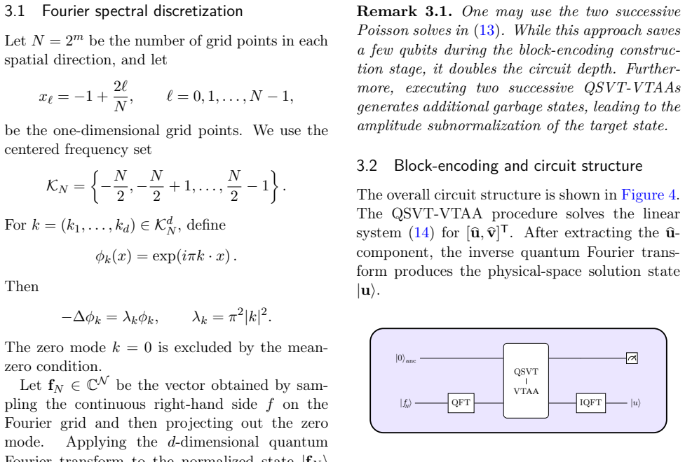


Reference graph
Works this paper leans on
-
[1]
V. V. Meleshko. Selected topics in the history of the two-dimensional biharmonic problem.Applied Mechanics Reviews56, 33– 85 (2003)
2003
-
[2]
Martinod, A
T. Martinod, A. Fierro, C. Posada, and J. J. Sanchez. On the biharmonic equation. Cuadernos de Ingeniería Matemática1(4) (2024)
2024
-
[3]
Ziegler.Mechanics of Solids and Fluids
F. Ziegler.Mechanics of Solids and Fluids. Springer, New York (1995). doi:10.1007/978- 1-4612-0805-1
doi:10.1007/978- 1995
-
[4]
H. Eschenauer, N. Olhoff, and W. Schnell. Applied Structural Mechanics: Fundamen- tals of Elasticity, Load-Bearing Structures, Structural Optimization. Springer, Berlin (1997). doi:10.1007/978-3-642-59205-8
-
[5]
J. D. Anderson, Jr.Computational Fluid Dynamics: The Basics with Applications. McGraw–Hill, New York (1995)
1995
- [6]
-
[7]
W. H. Press, S. A. Teukolsky, W. T. Vetterling, and B. P. Flannery.Numerical Recipes: The Art of Scientific Computing, 3rd ed. Cambridge University Press, Cam- bridge (2007)
2007
-
[8]
J. H. Argyris, I. Fried, and D. W. Scharpf. The TUBA family of plate elements for the matrix displacement method.Aeronautical Journal72, 701–709 (1968)
1968
-
[9]
K. Bell. A refined triangular plate bending finite element.International Journal for Nu- merical Methods in Engineering1, 101–122 (1969)
1969
-
[10]
F. K. Bogner, R. L. Fox, and L. A. Schmit. The generation of interelement-compatible stiffness and mass matrices by the use of in- terpolation formulas. InProceedings of the Conference on Matrix Methods in Structural Mechanics, pp. 397–444, Air Force Institute of Technology, Wright–Patterson Air Force Base, Ohio (1965)
1965
-
[11]
P. G. Ciarlet and P.-A. Raviart. A mixed finite element method for the biharmonic equation. In C. de Boor, ed.,Mathematical Aspects of Finite Elements in Partial Dif- ferential Equations, pp. 125–143. Academic Press, New York (1974). 23
1974
-
[12]
L. W. Ehrlich. Solving the biharmonic equa- tion as coupled finite difference equations. SIAM Journal on Numerical Analysis8, 278–287 (1971)
1971
-
[13]
P. E. Bjørstad. Fast numerical solution of the biharmonic Dirichlet problem on rectan- gles.SIAM Journal on Numerical Analysis 20, 59–71 (1983). doi:10.1137/0720004
-
[14]
J. W. Stephenson. Single cell discretiza- tions of order two and four for bihar- monic problems.Journal of Computational Physics55, 65–80 (1984). doi:10.1016/0021- 9991(84)90015-9
doi:10.1016/0021- 1984
-
[15]
A. W. Harrow, A. Hassidim, and S. Lloyd. Quantum algorithm for lin- ear systems of equations.Physical Review Letters103, 150502 (2009). doi:10.1103/PhysRevLett.103.150502
-
[16]
A. M. Childs, R. Kothari, and R. D. Somma. Quantum algorithm for systems of linear equations with exponentially im- proveddependenceonprecision.SIAM Jour- nal on Computing46, 1920–1950 (2017). doi:10.1137/16M1087072
- [17]
-
[18]
S. Jin and N. Liu. Quantum simulation of discrete linear dynamical systems and sim- ple iterative methods in linear algebra via Schrödingerisation.Proceedings of the Royal Society A: Mathematical, Physical and En- gineering Sciences480, 20230370 (2024). doi:10.1098/rspa.2023.0370
arXiv 2024
-
[19]
S. Jin, N. Liu, C. Ma, and Y. Yu. Quan- tum preconditioning method for finite dif- ference discretizations of the Poisson equa- tion via Schrödingerization.arXiv preprint arXiv:2505.06866v2(2026)
Pith/arXiv arXiv 2026
-
[20]
S. Chakraborty, A. Morolia, and A. Peduri. Quantum regularized least squares.Quan- tum7, 988 (2023). doi:10.22331/q-2023-04- 27-988
-
[21]
T. Kharazi, A. M. Alkadri, J.-P. Liu, K. K. Mandadapu, and K. B. Whaley. Explicit block encodings of boundary value problems for many-body elliptic operators.Quantum 9, 1764 (2025). doi:10.22331/q-2025-06-04- 1764
-
[22]
G. H. Low and I. L. Chuang. Opti- mal Hamiltonian simulation by quan- tum signal processing.Physical Re- view Letters118, 010501 (2017). doi:10.1103/PhysRevLett.118.010501
-
[23]
L. Lin. Lecture notes on quantum algorithms for scientific computation.arXiv preprint arXiv:2201.08309(2022). arXiv:2201.08309
Pith/arXiv arXiv 2022
-
[24]
M. Möttönen, J. J. Vartiainen, V. Bergholm, and M. M. Salomaa. Quantum circuits for general multiqubit gates.Physi- cal Review Letters93, 130502 (2004). doi:10.1103/PhysRevLett.93.130502
-
[25]
L. Lin. Mathematical and numerical analysis of quantum signal processing.arXiv preprint arXiv:2510.00443(2025). arXiv:2510.00443
arXiv 2025
-
[26]
C. Gidney. Halving the cost of quan- tum addition.Quantum2, 74 (2018). doi:10.22331/q-2018-06-18-74
-
[27]
Novikau and I
I. Novikau and I. Joseph. Estimating QSVT angles for matrix inversion with large con- dition numbers.Journal of Computational Physics525, 113767 (2025)
2025
-
[28]
Klappenecker and M
A. Klappenecker and M. Rötteler. Discrete cosine transforms on quantum computers. InProceedings of the Second International Symposium on Image and Signal Processing and Analysis, pp. 464–468 (2001)
2001
-
[29]
A. A. Zecchi, C. Sanavio, L. Cappelli, S. Perotto, A. Roggero, and S. Succi. Block encoding of sparse matrices with a pe- riodic diagonal structure.arXiv preprint arXiv:2602.10589(2026). arXiv:2602.10589
arXiv 2026
-
[30]
J. H. Bramble. A second order finite differ- ence analog of the first biharmonic bound- ary value problem.Numerische Mathematik 9, 236–249 (1966). doi:10.1007/BF02162087
-
[31]
Saad.Iterative Methods for Sparse Linear Systems, 2nd ed
Y. Saad.Iterative Methods for Sparse Linear Systems, 2nd ed. SIAM, Philadelphia (2003). doi:10.1137/1.9780898718003
-
[32]
G. H. Golub and C. F. Van Loan.Matrix Computations, 4th ed. Johns Hopkins Uni- versity Press, Baltimore (2013)
2013
-
[33]
W. Heinrichs. A stabilized treatment of the biharmonic operator with spectral meth- ods.SIAM Journal on Scientific and Sta- tistical Computing12, 1162–1172 (1991). doi:10.1137/0912061
-
[34]
B. Bialecki and A. Karageorghis. A Legen- 24 dre spectral Galerkin method for the bihar- monic Dirichlet problem.SIAM Journal on Scientific Computing22, 1549–1569 (2000). doi:10.1137/S1064827598342407
-
[35]
UnitaryLab 2.0.https:// test-studio.UnitaryLab.com/
UnitaryLab. UnitaryLab 2.0.https:// test-studio.UnitaryLab.com/. Accessed May 21, 2026. 25
2026
discussion (0)
Sign in with ORCID, Apple, or X to comment. Anyone can read and Pith papers without signing in.