REVIEW 3 major objections 8 minor 48 references
Integral Hilbert spaces and the dynamics of loop quantum cosmos
T0 review · 3 major / 8 minor · reviewed 2026-08-15 · deepseek-v4-flash
Pith's one-line read This paper claims that integral superselection-sector states preserve the semiclassical properties of single-sector states, within numerical precision, making the integral Hilbert space a viable replacement in this model.
desk verdict A careful, honest numerical test of the integral Hilbert space construction in one LQC model; the central claim holds for what is actually probed, but the headline conclusion is narrower than the paper's wording suggests. read the letter →
The pith
A machine-rendered reading of the paper's core claim, the machinery that carries it, and where it could break.
The reading
What carries the argument
The load-bearing object is the LQC evolution operator $\Theta_\Lambda = \Theta_o - \pi G \gamma^2 \Delta \Lambda v^2\,\mathbb{1}$, a second-order difference operator on each superselection lattice $\mathcal{L}_\epsilon = \epsilon + 4\mathbb{Z}$. Its non-negative spectrum $\{\omega_j^2\}$ supplies the energy basis $e_{\epsilon,j}$ used in the Gaussian spectral profiles. The integral Hilbert space construction $\mathcal{H}_{\mathrm{int}} = \frac{1}{4}\int_0^4 \mathcal{H}_\epsilon\, d\epsilon$ is what makes the nonseparable kinematical space separable without choosing a sector. The paper's test proceeds by comparing the volume expectation $\langle V\rangle$ and variance $\Delta V$ computed from single-sector states versus sector-integrated states, using two numerical routes to the same spectrum: the problem-specific shots method and a standard tridiagonal eigensolver.
What would settle it
Compute the volume trajectories with a basis accurate to better than $10^{-15}$ over the full range of $\epsilon$ and $\phi$, using a non-Gaussian spectral profile or an observable beyond the volume; if the sector-averaged variance then grows monotonically with $\phi$ or the relative difference $\delta\sigma_r$ exceeds $10^{-9}$ away from recollapse points, the paper's claim of no added decoherence would be refuted.
Extended reading notes
Core claim
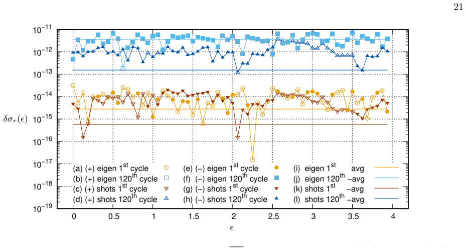
On the paper's own terms, the discovery is that integrating over superselection sectors does not spoil the semiclassical dynamics of the example universe. The integral Hilbert space $\mathcal{H}_{\mathrm{int}} = \frac{1}{4}\int_0^4 \mathcal{H}_\epsilon\, d\epsilon$ is separable and carries a well-defined action of observables through their restrictions to each sector. For the flat isotropic model with $\Lambda<0$ and a massless scalar, the authors compute the spectra of the evolution operator $\Theta_\Lambda$ on 64 sectors using two independent numerical methods, form Gaussian spectral profiles peaked at $\omega_0 = 10^3$ and $4\cdot 10^3$ (in $G^{1/2}$) with two variances, for four values of $\Lambda$, and evolve the volume expectation value and variance through $\phi \in [0,160]\,G^{-1/2}$. They report that relative differences between integral and single-sector trajectories stay below $10^{-9}$ throughout, that the slow growth of the apparent difference falls by several orders of magnitude when the basis is computed in higher precision, and that the averaged variance difference oscillates around zero rather than trending, so there is no detectable extra decoherence. The two methods' spectra agree to relative differences near $10^{-14}$, and the standard eigensolver is at least as accurate while being much easier to apply, at the cost of an order of magnitude more computation.
Load-bearing premise
The comparison treats semiclassicality as meaning small variance of the volume operator for Gaussian spectral profiles with a handful of parameters; if other observables, higher moments, or non-Gaussian states would reveal sector-induced spreading, the conclusion could fail.
Editorial extensions
If this is right
- In this model, the integral Hilbert space can replace single-sector projections: the volume dynamics of semiclassical states is unchanged within numerical precision, so no sector selection is needed.
- The standard eigensolver reproduces the dedicated shots method's spectra to about $10^{-14}$ relative agreement, so future studies can use generic numerical libraries rather than problem-specific code.
- The apparent small growth of differences between integral and single-sector states over time is numerical, not physical; increasing basis precision reduces it by several orders of magnitude.
- Because the eigenvalue curves $\omega_j(\epsilon)$ vary continuously with $\epsilon$, the integral Hilbert space supports a continuous range of energies, whereas each sector alone has a discrete spectrum.
- The paper stresses that the result is model-specific: extending the conclusion to models whose sectors already have continuous spectra or non-trivial measure spaces is not automatic.
Reading between the lines
- A natural extension would be to probe semiclassicality with observables other than the volume operator, such as the Hubble parameter or bounce-time moments, and with non-Gaussian spectral profiles; if those also show no sector-induced differences, the conclusion would be much stronger.
- The paper leaves open whether the integral construction remains well-behaved when the individual sectors have continuous spectra; one concrete test would be an anisotropic model like Bianchi I where this is the actual obstacle.
- The recollapse-point spikes in the shots method suggest that tail extrapolation, not the physics, is the limiting error source; replacing the exponential tail extrapolation with the exact decay of the corresponding continuum-geometry eigenfunctions would likely eliminate them and make the dedicated method competitive in accuracy at high $\omega_0$.
- The success of the integral construction here hints that superselection sectors are not physically distinguished: the dynamics averaged over them is the same, so observables may be definable without ever choosing a sector.
Signed reviews
Editorial analysis
A structured set of objections, weighed in public.
Referee Report
Summary. The paper studies the integral superselection-sector Hilbert space construction of Barbero et al. in the concrete LQC model of a flat isotropic universe with a negative cosmological constant and a massless scalar field. It computes the spectrum of the evolution operator Θ_Λ by two independent numerical methods—the purpose-built "shots" method of earlier work and a direct application of the Eigen library—and compares the volume expectation values and variances of Gaussian semiclassical states evolved over many bounce–recollapse cycles, in single-sector and integral-sector constructions. The main reported finding is that, within numerical precision, the integral states preserve the volume semiclassicality properties of single-sector states and show no observable increase of decoherence; a secondary finding is that the standard eigensolver reproduces and in most cases improves on the dedicated shots method, at the price of significantly larger computational resources.
Significance. If correct, the central numerical result provides direct evidence that the integral Hilbert space can serve as a practical replacement for single-sector projections in models where the latter are intractable, while the method comparison validates the older shots code and demonstrates that standard numerical libraries are usable for this class of problems. The paper is a numerical case study rather than a theorem; its strengths are the use of two independent implementations, the precision-escalation check (double vs long double), the explicit parameter scan over Λ, ω_o, σ_ω and 64 sectors, and the clear statement of model-specific limitations in Sec. V. The main claims are therefore plausible but rest on a fairly narrow set of observables and states, which is the central point needing attention.
major comments (3)
- [Sec. IVA, Eqs. (19)–(22)] The manuscript never states whether the discrete spectral coefficients obtained by sampling the Gaussian profile (20) are renormalized in each superselection sector. Because the spectra of Θ_Λ differ across ϵ, the sums ∑_j |Ψ̃_ϵ,j|² are not automatically equal, and if the sector states are not unit-normalized the objects in (21) are not expectation values; the comparison of δV_r and δσ_r in (23) would then mix normalization fluctuations with physical sector differences. Please specify the normalization procedure and confirm that every sector state entering the integrals in (22) has unit norm.
- [Sec. IVB and Sec. V] The conclusion that "there is no noticeable increase of decoherence due to differences between sectors" is drawn from the first two moments of a single observable, the volume, for Gaussian spectral profiles with ω_o ∈ {1000, 4000} G^{1/2}, σ_ω ∈ {50/√2, 200/√2} G^{1/2}, and Λ ∈ {-0.2, -0.1, -0.05, -0.01} l_Pl^{-2}. This diagnostic cannot exclude sector-induced broadening of the momentum-conjugate observable b, growth of higher cumulants of V, or qualitatively different behavior for non-Gaussian or much wider profiles. Since the abstract phrases the result as a general statement about "long term semiclassicality properties," the claim should either be restricted to the volume-moment criterion used here or supported by additional probes.
- [Sec. IIIC, Sec. IIID, and Fig. 9] The independent validation of the eigenlibrary basis against the shots method is shown for the first 3000 eigenvalues in three sectors, but the most demanding dynamical runs (ω_o = 4000, Λ = -0.05) require about 3400 eigenvalues per sector (Sec. IIID). The accuracy of eigenpairs 3001–3400 is therefore not directly benchmarked, and since truncation and boundary errors typically increase with eigenvalue, this is precisely the range where the "lowest 10%" assumption is least safe. Please extend the comparison to the full set of eigenvalues used in the dynamics or provide an explicit error estimate for that range.
minor comments (8)
- [Sec. IVB, point 1] The text states that the evolution is performed within the range ϕ ∈ [0,160] G^{-1/2}, but all figures and the discussion of the 120th cycle correspond to ϕ up to 60000 G^{-1/2} (e.g., Fig. 3); this inconsistency should be corrected.
- [Abstract and Sec. IIID/Conclusions] The abstract describes the Eigen-based method as "more efficient" than the shots method, but Sec. IIID and the Conclusions state that the new method requires at least an order of magnitude more computational resources; recommend rewording to "easier to apply" or "more accurate in most cases".
- [Eqs. (23) and (24)] The symbol δσ_r is used both for the sector-resolved quantity δσ_r(ϵ,ϕ) in (23) and for the sector-averaged quantity δσr(ϕ) in (24); please use distinct notation to avoid confusion.
- [Sec. IIIB] The word "bissection" should be "bisection" in the two places where it appears.
- [Sec. V] The word "relatiely" should be "relatively".
- [References] Reference [24] is missing the article number and page range; it should be Phys. Rev. D 77, 124025 (2008).
- [Figs. 6 and 7 captions] The captions use "(+)" and "(−)" without explaining that these denote the positive and negative branches of the plotted quantity; the captions should be self-contained.
- [Sec. II and Introduction] The name "Friedman-Lemaitre-Robertson-Walker" should be "Friedmann-Lemaître-Robertson-Walker," and the inconsistent use of "FRLW" versus "FLRW" should be unified.
Circularity Check
No significant circularity: the central numerical comparison is self-contained, with only minor reliance on the authors' prior construction of integral Hilbert spaces.
full rationale
The paper's central claim, that integral superselection-sector states preserve the semiclassical properties of single-sector states, is established by direct numerical simulation, not by construction. Equation (22) does define the integral expectation values as averages of sector expectation values via Eq. (13), but the paper does not present that averaging identity as a prediction; the nontrivial content is the behavior of the variance ΔV and of the relative difference δσ_r, which depends on the spread of sector mean volumes and is not forced by any equation. The numerical spectra are obtained by two independent methods, the older shots method [24] and the standard Eigen library, and their mutual agreement (Fig. 9, relative differences ~1e-14) provides an external consistency benchmark. Prior self-citations ([22], [24], [28]) supply the model setup and the integral-Hilbert-space construction, but the conclusion that there is no increased decoherence is a new numerical result with stated model-specific limitations in Sec. V. No fitted parameter is renamed as a prediction, no uniqueness theorem is imported from the authors, and no ansatz is smuggled in as a load-bearing substitute for computation. The only soft spot, namely probing semiclassicality through volume mean and variance for Gaussian states, is a scope limitation rather than a circular step.
Assumptions & free parameters
free parameters (4)
- Λ =
-0.2, -0.1, -0.05, -0.01 ℓ_Pl^{-2}
- ω_o =
10^3, 4×10^3 G^{1/2}
- σ_ω =
50/√2, 200/√2 G^{1/2}
- integration grid sectors =
64
assumptions (5)
- domain assumption The polymer representation and Thiemann regularization produce the difference operator Θ_Λ in Eq. (7) with superselection sectors L_ϵ = ϵ + 4Z preserved by its action.
- domain assumption The integral Hilbert space H_int in Eq. (12), with Lebesgue measure over ϵ and observable action via Eq. (13), is a valid separable Hilbert space, and equivalent choices of measure yield unitarily equivalent spaces.
- domain assumption The spectrum of Θ_Λ is purely discrete and nondegenerate for each superselection sector, so the Gaussian spectral profile (20) defines normalizable states.
- ad hoc to paper Truncating Θ_Λ to a finite matrix introduces an infinite potential barrier at the boundary, but for a sufficiently large matrix the lowest 10% of eigenpairs remain accurate.
- domain assumption Normalizable eigenfunctions are identified by sign flips of growing exponential tails in the shots method, and decaying tails are extrapolated exponentially.
Cite this review
Pith. "Pith review of Integral Hilbert spaces and the dynamics of loop quantum cosmos." pith.science (2026). https://pith.science/paper/TUCX436E
@misc{pith2026260802798,
  author       = {Pith},
  title        = {Pith review of: Integral Hilbert spaces and the dynamics of loop quantum cosmos},
  year         = {2026},
  howpublished = {\url{https://pith.science/paper/TUCX436E}},
  note         = {Machine review of arXiv:2608.02798}
}
read the original abstract
Polymer quantization program applied in Loop Quantum Gravity/Cosmology leads to nonseparable Hilbert spaces. Commonly, one sidesteps this problem by singling out and working with a separable superselection sector. This is however often no longer accessible in more involved models beyond isotropic ones. In an alternative approach one builds a separable Hilbert space as an integral over all available sectors. Here we test the dynamics following from the latter on the example of a flat isotropic Universe admitting negative cosmological constant and a massless scalar field. There, numerical evolution of (initially) semiclassical states shows that there is no relevant difference in their long term semiclassicality properties in comparison to those in a single sector approach. Further, the older (problem-specific) numerical methods are compared against an application of more common and more efficient standard tools (eigen library).
Figures


Figures from the paper (9 more)




Reference graph
Works this paper leans on
-
[1]
The kernel ofˆNChas been found by group averaging procedure (see [33]). The physical Hilbert space is spanned by the states represented (in volume and scalar field representation) by the wave functions3 Ψ(v,ϕ) = ∞∑ k=0 ˜Ψnen(v)eiωnϕ ,(11) whereω 2 n weretheelementsofthespectrumofΘ λ (whichinthiscaseispurelydiscreteandnondegenerate), en are the normalized ...
-
[2]
In order to define a nontrivial dynamics the notion of partial observables [34, 35] was used. Specifically, the fieldϕhasbeenconsideredasanevolutionparameterandsubsequentlythesetofobservablescorresponding to values of geometry observables at a given valueϕhas been constructed. The strict procedure of constructing such family is described for example in [3...
-
[3]
Let us now consider an alternative to choosing a single superselection sectorHω
Once both physical states and a sufficiently large set of physically interesting observables were available, a set of semiclassical states (in particular in [24] appropriate cutoffs of Gaussian spectral profiles toSp(ΘΛ)) has been selected and the quantum trajectories (expectation values of the observables as functions ofϕ) were evaluated. Let us now cons...
-
[4]
4A), in the middle of expansion (Fig
Across allϵsectors the relative difference of volume stays almost the same, within the range of numerical error, as shown on Figure 4, which shows a horizontal cross section of these colormaps done at bounce 11 (Fig. 4A), in the middle of expansion (Fig. 4B), at recollapse (Fig. 4C) and in the middle of contraction (Fig. 4D). Across all sectors the value ...
-
[5]
The relative differences(δVr,δσr)remained smaller than10−9 throughout the evolution (performed within the rangeϕ∈[0,160]G −1/2) independently of the method used, as it can be seen in Fig. 3. There, the left part of Fig. 3 shows the expectation value⟨V⟩over several bounce-recollapse cycles, the middle colormap shows the relative differenceδVr(ϵ,ϕ)and the r...
-
[6]
As the state evolves (ϕincreases) one observes a slight increase of|δVr|and|δσ r|, however the comparison of the results calculated with use of basis generated with a different precision shows, that this increase should be attributed to the numerical error. This is shown in Fig. 5, where the evaluation of the relative differencesδV r andδσ r with use of b...
-
[7]
When the basis is generated byeigenlibrary (top row in Fig. 3) the relative differences are in fact smaller than10−11, while the old shots method (bottom row in Fig. 3) has visible sharp peaks (the yellow-green horizontal lines on both colormaps) corresponding to points of recollapse, which amounts to increase of the differences to10−9. A vertical cross-s...
-
[8]
E. Alesci and F. Cianfrani, Phys. Rev. D87, 083521 (2013), arXiv:1301.2245 [gr-qc]; E. Alesci, F. Cianfrani, and C. Rovelli, Phys. Rev. D88, 104001 (2013), arXiv:1309.6304 [gr-qc]; E. Alesci and F. Cianfrani, Phys. Rev. D90, 024006 (2014), arXiv:1402.3155 [gr-qc]
arXiv 2013
Show all 48 references
-
[9]
Indeed, the analysis of the averaged relative difference δσr(ϕ) := 1 4 ∫4 0 δσr(ϵ,ϕ)dϵ(24) shows no particular trend in its behavior
The integral states do not show any detectable increase in variance of volume throughout the evolution in comparison to single sector ones. Indeed, the analysis of the averaged relative difference δσr(ϕ) := 1 4 ∫4 0 δσr(ϵ,ϕ)dϵ(24) shows no particular trend in its behavior. Hav...
-
[10]
Indeed, the comparison of the eigenvalues ofˆΘΛ evaluated byeigenlibrary and shots method shows an agreement to within the10−14 relative difference
The results computed with use of bases generated via different methods are consistent. Indeed, the comparison of the eigenvalues ofˆΘΛ evaluated byeigenlibrary and shots method shows an agreement to within the10−14 relative difference. This can be seen in Fig. 9, which shows t...
2020
-
[11]
Rovelli,Quantum gravity, Cambridge Monographs on Mathematical Physics (Univ
C. Rovelli,Quantum gravity, Cambridge Monographs on Mathematical Physics (Univ. Pr., Cambridge, UK, 2004)
2004
-
[12]
Thiemann, Modern Canonical Quantum General Relativity, Cambridge Monographs on Mathematical Physics (Cambridge University Press, 2007)
T. Thiemann, Modern Canonical Quantum General Relativity, Cambridge Monographs on Mathematical Physics (Cambridge University Press, 2007)
2007
-
[13]
Ashtekar and J
A. Ashtekar and J. Lewandowski, Class. Quant. Grav.21, R53 (2004), arXiv:gr-qc/0404018
2004 arXiv
-
[14]
Domagala, K
M. Domagala, K. Giesel, W. Kaminski, and J. Lewandowski, Phys. Rev. D82, 104038 (2010), arXiv:1009.2445 [gr-qc]
2010 arXiv
-
[15]
Husain and T
V. Husain and T. Pawlowski, Phys. Rev. Lett.108, 141301 (2012), arXiv:1108.1145 [gr-qc]
2012 arXiv
-
[16]
Giesel and T
K. Giesel and T. Thiemann, Class. Quant. Grav.32, 135015 (2015), arXiv:1206.3807 [gr-qc]
2015 arXiv
-
[17]
Zhang, J
C. Zhang, J. Lewandowski, H. Li, and Y. Ma, Phys. Rev. D99, 124012 (2019), arXiv:1904.07046 [gr-qc]
2019 arXiv
-
[18]
Martin-Benito, G
M. Martin-Benito, G. A. Mena Marugan, and T. Pawlowski, Phys. Rev. D78, 064008 (2008), arXiv:0804.3157 [gr-qc]; M. Martin-Benito, G. A. M. Marugan, and T. Pawlowski, Phys. Rev. D80, 084038 (2009), arXiv:0906.3751 [gr-qc]
2008 arXiv
-
[19]
Bilski, E
J. Bilski, E. Alesci, F. Cianfrani, P. Donà, and A. Marcianò, Phys. Rev. D95, 104048 (2017), arXiv:1612.00324 [gr-qc]
2017 arXiv
-
[20]
Bojowald and R
M. Bojowald and R. Swiderski, Class. Quant. Grav.21, 4881 (2004), arXiv:gr-qc/0407018; M. Bojowald, Class. Quant. Grav.21, 3733 (2004), arXiv:gr-qc/0407017
2004 arXiv
-
[21]
Gambini, J
R. Gambini, J. Olmedo, and J. Pullin, Int. J. Mod. Phys. D25, 1642006 (2016), arXiv:1605.00969 [gr-qc]; Class. Quant. Grav.37, 205012 (2020), arXiv:2006.01513 [gr-qc]. 15
2016 arXiv
-
[22]
D. M. de Blas, J. Olmedo, and T. Pawłowski, Phys. Rev. D96, 106016 (2017), arXiv:1706.05673 [gr-qc]
2017 arXiv
-
[23]
Ashtekar and P
A. Ashtekar and P. Singh, Class. Quant. Grav.28, 213001 (2011), arXiv:1108.0893 [gr-qc]
2011 arXiv
-
[24]
Bojowald, Living Rev
M. Bojowald, Living Rev. Rel.11, 4 (2008)
2008
-
[25]
J. F. Barbero G., J. Prieto, and E. J. S. Villaseñor, Class. Quant. Grav.30, 165011 (2013), arXiv:1305.5406 [gr-qc]
2013 arXiv
-
[26]
Ashtekar, S
A. Ashtekar, S. Fairhurst, and J. L. Willis, Class. Quant. Grav.20, 1031 (2003), arXiv:gr-qc/0207106
2003 arXiv
-
[27]
finite box
for details). The quantization of this system in the framework of LQC has been described in details in [24], though here we introduce slight modifications following [28] (which will be discussed further on). Since the system admits a constraint –the Hamiltonian one– NC=p 2 ϕ−3...
-
[28]
Bojowald, Class
M. Bojowald, Class. Quant. Grav.20, 2595 (2003), arXiv:gr-qc/0303073; M. Bojowald, G. Date, and K. Vandersloot, Class. Quant. Grav.21, 1253 (2004), arXiv:gr-qc/0311004
2003 arXiv
-
[29]
Diener, A
P. Diener, A. Joe, M. Megevand, and P. Singh, Class. Quant. Grav.34, 094004 (2017), arXiv:1701.05824 [gr-qc]
2017 arXiv
-
[30]
Ashtekar and E
A. Ashtekar and E. Wilson-Ewing, Phys. Rev. D79, 083535 (2009), arXiv:0903.3397 [gr-qc]
2009 arXiv
-
[31]
Martin-Benito, L
M. Martin-Benito, L. J. Garay, G. A. Mena Marugan, and E. Wilson-Ewing, J. Phys. Conf. Ser.360, 012031 (2012), arXiv:1110.1941 [gr-qc]
2012 arXiv
-
[32]
J. F. Barbero G., T. Pawlowski, and E. J. S. Villasenor, Phys. Rev. D90, 067505 (2014), arXiv:1403.2974 [gr-qc]
2014 arXiv
-
[33]
Reed and B
M. Reed and B. Simon,Methods of Modern Mathematical Physics. vol.4: Analysis of Operators (Academic Press, 1978)
1978
-
[34]
Bentivegna and T
E. Bentivegna and T. Pawlowski, Physical Review D77, 10.1103/physrevd.77.124025 (2008)
2008 doi
-
[35]
G. A. Mena Marugan, J. Olmedo, and T. Pawlowski, Phys. Rev. D84, 064012 (2011), arXiv:1108.0829 [gr-qc]
2011 arXiv
-
[36]
J. F. Barbero G., Phys. Rev. D51, 5507 (1995), arXiv:gr-qc/9410014
1995 arXiv
-
[37]
Ashtekar, T
A. Ashtekar, T. Pawlowski, and P. Singh, Phys. Rev. D74, 084003 (2006), arXiv:gr-qc/0607039
2006 arXiv
-
[38]
Pawłowski and A
T. Pawłowski and A. Ashtekar, Physical Review D85, 10.1103/physrevd.85.064001 (2012)
2012 doi
-
[39]
Ashtekar, A
A. Ashtekar, A. Corichi, and P. Singh, Phys. Rev. D77, 024046 (2008), arXiv:0710.3565 [gr-qc]
2008 arXiv
-
[40]
Ashtekar, M
A. Ashtekar, M. Bojowald, and J. Lewandowski, Adv. Theor. Math. Phys.7, 233 (2003), arXiv:gr-qc/0304074
2003 arXiv
- [41]
-
[42]
Kowalczyk and T
M. Kowalczyk and T. Pawłowski, Phys. Rev. D108, 086010 (2023), arXiv:2212.12527 [gr-qc]
2023 arXiv
-
[43]
Ashtekar, J
A. Ashtekar, J. Lewandowski, D. Marolf, J. Mourao, and T. Thiemann, J. Math. Phys.36, 6456 (1995), arXiv:gr- qc/9504018
1995
- [44]
- [45]
-
[46]
Kaminski, J
W. Kaminski, J. Lewandowski, and T. Pawlowski, Class. Quant. Grav.26, 245016 (2009), arXiv:0907.4322 [gr-qc]
2009 arXiv
-
[47]
Singh and K
P. Singh and K. Vandersloot, Phys. Rev. D72, 084004 (2005), arXiv:gr-qc/0507029
2005 arXiv
-
[48]
Guennebaud, B
G. Guennebaud, B. Jacob,et al., Eigen v3,http://eigen.tuxfamily.org(2010). 16 -4 -3 -2 -1 0 1 2 3 4 0 1000 2000 3000 4000 5000 6000 7000 v ψω ω=300.4507 ω=300.3507 ω=300.5507 Figure 1. An illustration of the shots method functionality for the exceptional sectorϵ= 0on the examp...
2010
Reviewed August 15, 2026 · model on record in the stance chip above.
Discussion (0). Continue with ORCID to comment.