REVIEW 4 major objections 5 minor 61 references
Variational Parameter Calibration with Physics-Aware Latent-Space Surrogates
T0 review · 4 major / 5 minor · reviewed 2026-08-15 · deepseek-v4-flash
Pith's one-line read The paper argues that adding observable supervision to a latent-space surrogate—training the latent code to predict physical parameters—produces a differentiable observation operator whose variational parameter calibration is generally…
desk verdict A solid, carefully built empirical paper on differentiable latent-space surrogates for variational calibration; the relative OACAE-vs-CAE ablation is convincing, but the absolute physical-calibration claim is only checked through the surrogate itself. read the letter →
The pith
A machine-rendered reading of the paper's core claim, the machinery that carries it, and where it could break.
The reading
What carries the argument
The load-bearing object is the observable-augmented convolutional autoencoder (OACAE) with its parameter-to-latent regressor, forming the surrogate observation operator $H(\theta_{\mathrm{control}}) = F_d^r(E_b(\theta_{\mathrm{control}}, \theta^{\mathrm{fixed}}_{t_k}))$, where $F_d^r$ is the frozen decoder and $E_b$ is an MLP regressor. Training happens in two phases: the first minimizes $L^r_1 = \|x-\hat{x}^r\|_2^2 + \alpha\|\theta-\hat{\theta}\|_2^2$, which couples the latent code to the parameters; the second, with encoder and decoder frozen, trains $E_b$ by minimizing $L^r_2 = \|x-\hat{x}^{r,*}\|_2^2 + \beta\|z^r - z^{r,*}\|_2^2$. This two-phase construction makes the whole parameter-to-observation map differentiable in $\theta$, so the 3D-Var and 4D-Var cost functions can be minimized by gradient descent through the network, while the observable-supervision term is what pushes the latent space to separate parameter regimes and evolve smoothly in time. A second phase-sensitive component is the case-level split of training and test data, which tests generalization to unseen parameter configurations.
What would settle it
Run an independent high-fidelity CFD solver at the parameters returned by OACAE-MLP 3D-Var and compare those flow fields with fields obtained at the true parameters and at CAE-MLP-calibrated parameters; if the OACAE-calibrated fields are not consistently closer to the true dynamics, the calibration advantage does not generalize beyond the surrogate. A second check is to perturb a parameter direction the surrogate resolves poorly and observe whether the optimizer drifts to a compensating parameter value, which would indicate that the objective rewards surrogate self-consistency rather than physical fidelity.
Extended reading notes
Core claim
The central claim is that reconstruction accuracy is the wrong selection criterion for surrogates used in inverse problems. A standard autoencoder trained only to reconstruct fields can leave parameter-sensitive directions poorly organized in its latent space, so its downstream calibration is unstable even when its predictions look accurate. The paper's proposed fix is observable supervision: during autoencoder training, a regression branch maps the latent code back to the physical parameters, and the training loss includes a term penalizing parameter-recovery error alongside field reconstruction. When this physics-aware autoencoder is frozen and coupled to a parameter-to-latent MLP, it forms an end-to-end differentiable surrogate whose variational assimilation consistently yields more concentrated parameter estimates around the true values than the reconstruction-only CAE-MLP ablation, with the advantage most visible under degraded observations.
Load-bearing premise
The calibration claim assumes the learned surrogate produces flow fields faithfully enough that the parameters minimizing the variational cost are close to the true physical parameters; the paper itself notes that true parameters need not minimize the surrogate-induced mismatch, so part of the measured improvement could be the surrogate compensating for its own bias.
Editorial extensions
If this is right
- The same surrogate can serve as observation operator in both 3D-Var and 4D-Var, so calibration becomes a gradient-based optimization over a few control parameters rather than repeated ensemble sampling.
- Because OACAE latent trajectories are more separated by parameter case and smoother in time, multi-time-step 4D-Var inherits better temporal consistency and yields lower long-horizon prediction error than the reconstruction-only ablation.
- Calibration under noisy, low-resolution, randomly masked, and block-wise partial observations remains accurate for OACAE-MLP, with the exception of regimes where the observations contain too little parameter-sensitive information.
- The reported online runtime of the variational DL-ROM approach scales better than the EnKF-POD-GPR baseline as the number of assimilated snapshots grows.
- Reconstruction quality alone ranks the three surrogates in the opposite order from calibration quality: POD is best at reconstruction but worst as an inverse surrogate.
Reading between the lines
- Editorial inference: the latent separability ratio $R_{\mathrm{sep}}$ reported for OACAE could be used as a cheap offline screen for whether a learned latent space will support inverse calibration, before variational assimilation is run.
- Editorial inference: if the result transfers, then for other parametric PDE inverse problems the same recipe—add a parameter-regression branch to any autoencoder-based surrogate—may improve identifiability even when pure reconstruction accuracy suffers slightly.
- Editorial inference: because the paper's consistency check compares the true and calibrated parameters through the surrogate's own observation mismatch, a stronger test against an independent full-order solver would reveal whether calibrated parameters remain faithful when the surrogate has structured bias.
- Editorial inference: the temporal-smoothness benefit suggests that extending the framework to latent-space dynamics, rather than including the time index as an input, could make 4D-Var work on longer or irregular observation windows.
Signed reviews
Editorial analysis
A structured set of objections, weighed in public.
Referee Report
Summary. The paper proposes a physics-aware reduced-order surrogate for variational parameter calibration of parametric flow systems. The method combines an observable-augmented convolutional autoencoder (OACAE) with an MLP parameter-to-latent regressor, yielding an end-to-end differentiable observation operator that is embedded into 3D-Var and 4D-Var cost functions. The authors compare this OACAE-MLP surrogate against a standard CAE-MLP surrogate and a POD-GPR-based EnKF baseline on the CFDBench dam-break and lid-driven cavity benchmarks. The central claim is that observable supervision improves calibration accuracy and reduces calibration variability relative to reconstruction-only surrogates, and that reconstruction accuracy alone is insufficient for inverse problems. The paper reports reconstruction/prediction metrics, single- and multi-time-step calibration results, a 44-case robustness study on dam flow, degraded-observation experiments, and sensitivity analyses for loss weights, latent dimension, learning rate, and covariance scaling.
Significance. If the central claim held in its full generality, the paper would make a useful contribution to surrogate-based data assimilation: it demonstrates an end-to-end differentiable pipeline, provides a controlled ablation isolating observable supervision, reports case-level data splitting to avoid leakage, and includes extensive sensitivity and robustness experiments. The 44-case study and degraded-observation tests are valuable. The paper also ships code and uses a public benchmark, which supports reproducibility. The main significance is therefore conditional: the evidence supports the two-parameter calibration claim, but the physical-space evaluation is partly circular, and the latent-space organization metrics are partly constructed by the training objective rather than measured independently.
major comments (4)
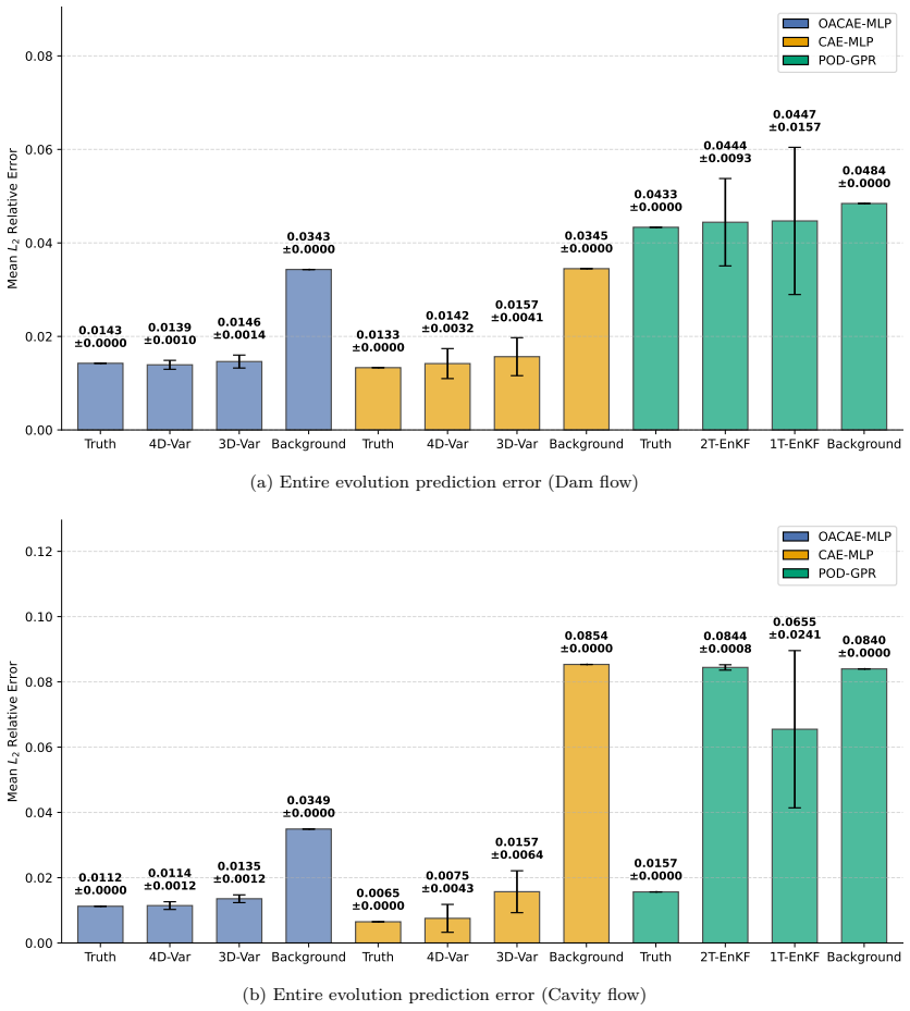
- [§3.6.1 and Figures 4, 6, 7] The physical-space validation is performed through the same learned surrogate or decoder that defines the inverse cost. The paper itself concedes in §3.6.1 that 'the true physical parameters do not necessarily minimize the surrogate-induced observation mismatch' and that a lower validation loss with analysis parameters is only a 'necessary consistency check.' Yet Figures 4, 6, and 7 use exactly this surrogate-induced observation mismatch or the surrogate decoder trajectory to support claims of improved physical-space prediction. These figures cannot distinguish physical calibration from bias compensation. The parameter-space MSEs in Tables 5–6 and Figure 9 are real mitigating evidence, but they cover only two calibrated parameters with the other parameters fixed at their true values. The absence of any full-order (ground-truth simulator) evaluation of the calibrated parameters is therefore a load-bearing gap. I recommend adding a full-order evaluation of a subset of calibrated parameters, or explicitly restricting the physical-space claims to surrogate-relative consistency.
- [Appendix D] The latent-space organization metrics in Appendix D are computed on the training set and are partly direct consequences of the observable-supervision loss in Eq. (13). The auxiliary branch E_a is trained to regress the parameters and the time index from the latent codes, so a larger separability ratio R_sep and smoother latent trajectories on the training set are expected outcomes of minimizing that regression loss, not independent evidence of a physically organized latent space. To support the claim that observable supervision yields a structurally different latent representation, the metrics should be reported on held-out test cases and compared against a control architecture with the same auxiliary branch capacity but without the observable-regression loss, or the claim should be weakened accordingly.
- [§3.2 and §3.3] The calibration experiments fix all but two physical parameters at their true values, and the preliminary multi-parameter assimilation tests that motivated this reduced control setting are described only narratively with no results. This restricts the central 'parameter calibration' claim to a two-parameter problem and leaves the identifiability-based selection of control parameters unreproducible. I ask the authors to report the preliminary multi-parameter tests (or an identifiability analysis) so that the reader can assess whether the two-parameter restriction is justified, or to revise the abstract and conclusions to state explicitly that the method is demonstrated only for two-parameter calibration.
- [Table 5 and §3.6.2] The headline single-case comparison in Table 5 is based on one selected evolution case per flow, and for each flow OACAE-MLP is worse than CAE-MLP on one of the two calibrated parameters (u_in for dam flow, ρ for cavity flow). The 44-case robustness study in Table 6 covers only dam flow. As a result, the evidence for the claim that OACAE-MLP 'generally reduces calibration error and variability' is substantially stronger for the dam u_in/h pair than for the cavity u_lid/ρ pair. I recommend reporting paired per-case statistics for the cavity flow test cases, or at least tempering the generalization claim about cavity-flow calibration.
minor comments (5)
- [§1.2] The text contains a typo: 'Typicaly examples include' should read 'Typical examples include.'
- [Eq. (9) and §2.2.2] The notation θ in Eq. (9) denotes 'the vector of physical observables' and includes the time index, which conflates physical parameters to be calibrated with the temporal label. This should be clarified, especially because the calibration cost functions in Eqs. (32)–(33) treat the time index as known and fixed.
- [§2.3.2] The sentence 'the reduced-order surrogate CAE-MLP serves as the observation operator H' refers back to a model introduced in different sections; the reference 'as defined in Section 3.2' should be updated to the correct methodological section.
- [§3.4 and Table 3] The claim that OACAE has 'slightly lower reconstruction accuracy' than CAE is supported, but the POD accuracy advantage is based on a 64×64 grid only; the authors should state more explicitly that this observation is dataset-specific and may not transfer to higher-resolution flows.
- [Appendix E.4 and Figure E.21] The covariance-scaling sensitivity analysis is described only for a single representative setting; reporting the range of calibration errors across multiple test cases would strengthen the robustness conclusion.
Circularity Check
Two supporting evaluations—latent-space organization metrics and 3D/4D-Var validation-loss comparisons—reduce to the fitted objectives by construction; the headline calibration-error claims retain independent ground-truth support.
-
self definitional
[Section 2.2.2, Eq. (13); Appendix D, Table D.10]
"we introduce a regression task Ea from the latent space to the parameter space: θ̂=Ea(zr;φa)... Lr1(φra,φre,φrd)=∥x−Frd(Fre(x;φre);φrd)∥22+α∥θ−Ea(Fre(x;φre);φra)∥22 ... Table D.10 reports the latent-space metrics on the training set. Compared with CAE, OACAE yields a smaller within-case variance and a substantially larger normalized separability ratio."
The OACAE latent codes are trained with the observable-regression term α∥θ−Ea(z)∥2, and θ includes the time index, so separation by parameter and temporal regularity are directly written into the training objective. Appendix D then computes R_sep, S(1), and S(2) on those same training-set latent codes. The reported improvement in separability and smoothness is therefore an expected consequence of the loss being minimized, not an independent discovery about the latent representation. It is a sanity check that the objective had its intended effect, not evidence that the latent space is physically meaningful beyond what the supervision loss enforces.
-
fitted input called prediction
[Section 3.6.1, Eqs. (32)-(33); Figures 4 and 6]
"Since the observation operator is a learned surrogate rather than the full-order model... the true physical parameters do not necessarily minimize the surrogate-induced observation mismatch. ... the effectiveness of variational data assimilation can be assessed through the 3D-Var validation loss, defined as the value of the observation term in the 3D-Var cost function... Overall, these results further demonstrate the effectiveness and enhanced robustness of the proposed physics-informed variational DA-DL-ROM framework for parameter calibration."
The analysis parameters are obtained by minimizing J3D-Var/J4D-Var (Eqs. 32-33) with the observation term dominating. Figures 4 and 6 then plot that same observation term evaluated at the analysis parameters versus the true parameters. By construction, the analysis is chosen to lower this term, so a lower or equal validation loss at the analysis point is a direct consequence of the optimization, not an independent confirmation of physical calibration. The paper itself labels the comparison only a 'necessary consistency check,' yet uses it to support the framework's effectiveness and robustness; the independent evidence is the ground-truth parameter-space error in Tables 5-6 and Figure 9.
full rationale
The paper's central calibration claim—that OACAE-MLP reduces parameter-estimation error relative to CAE-MLP and POD-GPR-EnKF—is not entirely circular: Tables 5-6 and Figure 9 compare estimated parameters against ground-truth values, which is external to the surrogate objective. Those experiments restrict calibration to two control parameters while fixing the others, but they still provide independent evidence. No load-bearing self-citation chain, imported uniqueness theorem, or ansatz-smuggling-via-citation pattern was found; the authors' own TorchDA software and external benchmarks are used as tools rather than as evidence for the main claim. However, two supporting analyses do reduce by construction. First, the Appendix D latent-organization metrics are computed on latent codes trained with a loss that directly regresses parameters and time, so higher separability and smoother trajectories are consequences of the fitted objective rather than independent validation. Second, the 3D/4D-Var validation-loss comparisons in Figures 4 and 6 use the same observation term that was minimized to obtain the analysis, making the lower loss at the analysis point a built-in property of the optimization; the paper explicitly concedes this is only a necessary consistency check. These by-construction evaluations do not destroy the external parameter-space evidence, but they do inflate the appearance of independent support for the physics-awareness claim, giving a partial circularity score of 6.
Assumptions & free parameters
free parameters (4)
- Observable-supervision weight alpha =
0.05
- Latent-supervision weight beta =
1
- Latent dimension q =
32
- Variational optimizer learning rate =
0.05 (3D-Var), 0.005 (4D-Var)
assumptions (6)
- domain assumption The high-fidelity snapshots in CFDBench are exact observations, and no model-error term is added to the variational cost.
- domain assumption The surrogate H(theta)=F_d(E_b(theta)) generalizes to held-out parameter configurations.
- ad hoc to paper The gradient of the surrogate-induced cost with respect to theta is a useful search direction for the true parameters.
- ad hoc to paper The temporal index is treated as an observable in E_a, so the latent space is also organized by time.
- domain assumption Weakly identifiable parameters can be fixed at ground truth without changing the conclusions.
- standard math SVD/POD, Gaussian process regression, and ensemble Kalman filter equations are applied as known methods.
Cite this review
Pith. "Pith review of Variational Parameter Calibration with Physics-Aware Latent-Space Surrogates." pith.science (2026). https://pith.science/paper/FLPBEZNT
@misc{pith2026260811435,
  author       = {Pith},
  title        = {Pith review of: Variational Parameter Calibration with Physics-Aware Latent-Space Surrogates},
  year         = {2026},
  howpublished = {\url{https://pith.science/paper/FLPBEZNT}},
  note         = {Machine review of arXiv:2608.11435}
}
read the original abstract
Forward and inverse modeling of parametric dynamical systems requires surrogate models that are not only accurate for state prediction, but also informative for parameter calibration. However, a systematic end-to-end differentiable formulation for coupling deep-learning-based reduced-order surrogates with variational parameter estimation remains underdeveloped. In this work, we introduce a physics-aware neural-network-based latent-space framework for reduced-order forward modeling and variational parameter estimation. The proposed autoencoder-based approach yields a differentiable surrogate that maps physical parameters to predicted flow fields through a latent representation. The observable supervision is used during offline training to encourage the latent variables to retain information correlated with system parameters, while the online inverse problem is solved in the parameter space through the surrogate-induced observation operator. The method is evaluated on two computational-fluid-dynamics benchmarks. The results show that reconstruction accuracy alone is insufficient for inverse modeling, owing to the lack of end-to-end differentiability or physics awareness for variational parameter calibration. Quantitative latent-space analysis further shows that observable supervision improves case-level separability and temporal organization of latent representations. Experiments with realistic measurement settings, including noisy, low-resolution, randomly masked, and block-wise partial observations, demonstrate the robustness of the proposed framework and show that it generally reduces calibration error and variability compared with the standard surrogate models.
Figures


Figures from the paper (8 more)




Reference graph
Works this paper leans on
-
[1]
R. N. Asl, Y. Yamazaki, K. Taghikhani,et al., “A physics-informed meta-learning frame- work for the continuous solution of parametric pdes on arbitrary geometries,”arXiv preprint arXiv:2504.02459, 2025
arXiv 2025
-
[2]
S. Burela, P. Krah, and J. Reiss, “Parametric model order reduction for a wildland fire model via the shifted pod-based deep learning method,”Adv. Comput. Math., vol. 51, no. 1, p. 9, 2025
work page 2025
-
[3]
S. Fresca, L. Dede’, and A. Manzoni, “A comprehensive deep learning-based approach to reduced order modeling of nonlinear time-dependent parametrized pdes,”J. Sci. Comput., vol. 87, no. 2, p. 61, 2021
work page 2021
-
[4]
K. Vlachas, T. Simpson, A. Garland,et al., “Reduced order modeling conditioned on monitored features for response and error bounds estimation in engineered systems,”Mech. Syst. Signal Process., vol. 226, p. 112261, 2025
work page 2025
-
[5]
G. K. Batchelor,An Introduction to Fluid Dynamics. Cambridge University Press, 1967
1967
-
[6]
L. D. Landau and E. M. Lifshitz,Fluid Mechanics. Pergamon Press, 1987
work page 1987
-
[7]
C. Dai, D. Yang, C. Zhang,et al., “Parameter identification of fluid field based on cfd reduced-order model and 3d-var data assimilation,”Ann. Nucl. Energy, vol. 219, p. 111459, 2025
work page 2025
-
[8]
Dynamic mode decomposition: Theory and applications,
J. H. Tu, “Dynamic mode decomposition: Theory and applications,” 2013
work page 2013
Show all 61 references
-
[9]
Ahybriddataassimilationanddynamicmodedecomposition approach for xenon dynamic prediction of nuclear reactor cores,
J.Liu, Z.Wang, Q.Li,et al., “Ahybriddataassimilationanddynamicmodedecomposition approach for xenon dynamic prediction of nuclear reactor cores,”Nucl. Sci. Eng., vol. 199, no. 6, pp. 888–906, 2025
2025
-
[10]
A kernel ridge regression combining nonlinear roms for accurate flow-field reconstruction with discontinuities,
W. Wang, C. Gong, X. Jia,et al., “A kernel ridge regression combining nonlinear roms for accurate flow-field reconstruction with discontinuities,”Aerosp. Sci. Technol., vol. 166, p. 110549, 2025
2025
-
[11]
Uncertainty-aware surrogate modeling for urban air pollutant dispersion prediction,
E. Lumet, M. C. Rochoux, T. Jaravel,et al., “Uncertainty-aware surrogate modeling for urban air pollutant dispersion prediction,”Build. Environ., vol. 267, p. 112287, 2025. 31
2025
-
[12]
A deep learning based approach to reduced or- der modeling for turbulent flow control using lstm neural networks,
A. T. Mohan and D. V. Gaitonde, “A deep learning based approach to reduced or- der modeling for turbulent flow control using lstm neural networks,”arXiv preprint arXiv:1804.09269, 2018
2018 arXiv
-
[13]
A graph convolutional autoencoder approach to model order reduction for parametrized pdes,
F. Pichi, B. Moya, and J. S. Hesthaven, “A graph convolutional autoencoder approach to model order reduction for parametrized pdes,”J. Comput. Phys., vol. 501, p. 112762, 2024
2024
-
[14]
Handling geometrical variability in nonlinear re- duced order modeling through continuous geometry-aware dl-roms,
S. Brivio, S. Fresca, and A. Manzoni, “Handling geometrical variability in nonlinear re- duced order modeling through continuous geometry-aware dl-roms,”Comput. Methods Appl. Mech. Eng., vol. 442, p. 117989, 2025
2025
-
[15]
Multi-level convolutional autoencoder networks for parametric prediction of spatio-temporal dynamics,
J. Xu and K. Duraisamy, “Multi-level convolutional autoencoder networks for parametric prediction of spatio-temporal dynamics,”Comput. Methods Appl. Mech. Eng., vol. 372, p. 113379, 2020
2020
-
[16]
Graspingextremeaerodynamicsonalow-dimensionalmanifold,
K. FukamiandK.Taira, “Graspingextremeaerodynamicsonalow-dimensionalmanifold,” Nat. Commun., vol. 14, no. 1, p. 6480, 2023
2023
-
[17]
Learning physics constrained dynamics using autoencoders,
T.-Y. Yang, J. Rosca, K. Narasimhan,et al., “Learning physics constrained dynamics using autoencoders,” inAdvances in Neural Information Processing Systems(S. Koyejo, S. Mohamed, A. Agarwal, D. Belgrave, K. Cho, and A. Oh, eds.), vol. 35, pp. 17157–17172, Curran Associates, Inc., 2022
2022
-
[18]
Observable-augmented manifold learning for multi-source tur- bulent flow data,
K. Fukami and K. Taira, “Observable-augmented manifold learning for multi-source tur- bulent flow data,”J. Fluid Mech., vol. 1010, p. R4, 2025
2025
-
[19]
Yuki algorithm and pod-rbf for elastostatic and dynamic crack identification,
B. Benaissa, N. A. Hocine, S. Khatir,et al., “Yuki algorithm and pod-rbf for elastostatic and dynamic crack identification,”J. Comput. Sci., vol. 55, p. 101451, 2021
2021
-
[20]
Deep neural network and yuki algorithm for inner damage characterization based on elastic boundary displacement,
N. Amoura, B. Benaissa, M. Al Ali,et al., “Deep neural network and yuki algorithm for inner damage characterization based on elastic boundary displacement,” inInternational Conference of Steel and Composite for Engineering Structures, pp.220–233, Springer, 2022
2022
-
[21]
Machine learning with data assimilation and uncertainty quantification for dynamical systems: A review,
S. Cheng, C. Quilodrán-Casas, S. Ouala,et al., “Machine learning with data assimilation and uncertainty quantification for dynamical systems: A review,”IEEE/CAA J. Autom. Sin., vol. 10, no. 6, pp. 1361–1387, 2023
2023
-
[22]
Bayesian inference of chaotic dynamics by merging data assimilation, machine learning and expectation-maximization,
M. Bocquet, J. Brajard, A. Carrassi,et al., “Bayesian inference of chaotic dynamics by merging data assimilation, machine learning and expectation-maximization,”Found. Data Sci., vol. 2, no. 1, p. 55–80, 2020
2020
-
[23]
M. Asch, M. Bocquet, and M. Nodet,Data Assimilation: Methods, Algorithms, and Ap- plications. Philadelphia, PA: Society for Industrial and Applied Mathematics, 2016
2016
-
[24]
Data assimilation in the geosciences: An overview of methods, issues, and perspectives,
A. Carrassi, M. Bocquet, L. Bertino,et al., “Data assimilation in the geosciences: An overview of methods, issues, and perspectives,”WIREs Clim. Chang., vol. 9, no. 5, p. e535, 2018
2018
-
[25]
The advantages of data assimi- lation in parametric space rather than classic grid space,
S. Dealbera, S. Raynaud, C. Granero Belinchon,et al., “The advantages of data assimi- lation in parametric space rather than classic grid space,”EGUsphere, vol. 2025, pp. 1–8, 2025
2025
-
[26]
Enkf data-driven reduced order assimilation system,
C. Liu, R. Fu, D. Xiao,et al., “Enkf data-driven reduced order assimilation system,”Eng. Anal. Bound. Elem., vol. 139, pp. 46–55, 2022. 32
2022
-
[27]
Generalised latent assimilation in heterogeneous reduced spaces with machine learning surrogate models,
S. Cheng, J. Chen, C. Anastasiou, P. Angeli, O. K. Matar, Y.-K. Guo, C. C. Pain, and R. Arcucci, “Generalised latent assimilation in heterogeneous reduced spaces with machine learning surrogate models,”Journal of Scientific Computing, vol. 94, no. 1, p. 11, 2023
2023
-
[28]
Multi-domain encoder–decoder neural networks for latent data assimilation in dynamical systems,
S. Cheng, Y. Zhuang, L. Kahouadji, C. Liu, J. Chen, O. K. Matar, and R. Arcucci, “Multi-domain encoder–decoder neural networks for latent data assimilation in dynamical systems,”Computer Methods in Applied Mechanics and Engineering, vol. 430, p. 117201, 2024
2024
-
[29]
Application and comparison of several adaptive sampling algorithms in reduced order modeling,
X. Liu, Z. Wang, H. Ji,et al., “Application and comparison of several adaptive sampling algorithms in reduced order modeling,”Heliyon, vol. 10, no. 15, 2024
2024
-
[30]
Surrogate-based ensemble data assimilation forreducinguncertaintyinlarge-eddysimulationofmicroscalepollutantdispersion,
E. Lumet, M. C. Rochoux, T. Jaravel,et al., “Surrogate-based ensemble data assimilation forreducinguncertaintyinlarge-eddysimulationofmicroscalepollutantdispersion,”Build. Environ., vol. 287, p. 113863, 2026
2026
-
[31]
Torchda: A python package for performing data assimila- tion with deep learning forward and transformation functions,
S. Cheng, J. Min, C. Liu,et al., “Torchda: A python package for performing data assimila- tion with deep learning forward and transformation functions,”Comput. Phys. Commun., vol. 306, p. 109359, 2025
2025
-
[32]
Cfdbench: A large-scale benchmark for machine learning methods in fluid dynamics,
Y. Luo, Y. Chen, and Z. Zhang, “Cfdbench: A large-scale benchmark for machine learning methods in fluid dynamics,”arXiv preprint arXiv:2310.05963, 2023
2023 arXiv
-
[33]
Surrogate-based bayesian inverse modeling of the hydrological system: An adaptive approach considering surrogate approximation error,
J. Zhang, Q. Zheng, D. Chen,et al., “Surrogate-based bayesian inverse modeling of the hydrological system: An adaptive approach considering surrogate approximation error,” Water Resour. Res., vol. 56, Jan. 2020
2020
-
[34]
Uncertainty quantification and propagation in surrogate-based bayesian inference,
P. Reiser, J. E. Aguilar, A. Guthke,et al., “Uncertainty quantification and propagation in surrogate-based bayesian inference,”Stat. and Comput., vol. 35, Mar. 2025
2025
-
[35]
Parametric probabilistic manifold decomposition for nonlinear model reduction,
J. Guo and D. Xiao, “Parametric probabilistic manifold decomposition for nonlinear model reduction,”arXiv preprint arXiv:2601.07278, 2026
2026
-
[36]
Bayesian gaussian process latent variable model,
M. Titsias and N. D. Lawrence, “Bayesian gaussian process latent variable model,” inPro- ceedings of the Thirteenth International Conference on Artificial Intelligence and Statistics (Y. W. Teh and M. Titterington, eds.), vol. 9 ofProceedings of Machine Learning Research, (Chi...
2010
-
[37]
Mechanics-informed autoencoder enables auto- mated detection and localization of unforeseen structural damage,
X. Li, H. Bolandi, M. Masmoudi,et al., “Mechanics-informed autoencoder enables auto- mated detection and localization of unforeseen structural damage,” 2024
2024
-
[38]
Physics-informed quantum neural network for solving forward and inverse problems of partial differential equations,
Y. Xiao, L. Yang, C. Shu,et al., “Physics-informed quantum neural network for solving forward and inverse problems of partial differential equations,”Phys. Fluids, vol. 36, no. 9, 2024
2024
-
[39]
Quantum machine learning for efficient reduced order mod- elling of turbulent flows,
H. Li, Y. Lou, and D. Xiao, “Quantum machine learning for efficient reduced order mod- elling of turbulent flows,” 2025
2025
-
[40]
Qcpinn: Quantum-classical physics-informed neural networks for solving pdes,
A. Farea, S. Khan, and M. S. Celebi, “Qcpinn: Quantum-classical physics-informed neural networks for solving pdes,” 2025
2025
-
[41]
Taflove,Computational electrodynamics the finite-difference time-domain method
A. Taflove,Computational electrodynamics the finite-difference time-domain method. 1995
1995
-
[42]
H. K. Versteeg and W. Malalasekera,An Introduction to Computational Fluid Dynamics: The Finite Volume Method. Pearson Education, 2007
2007
-
[43]
O. C. Zienkiewicz, R. L. Taylor, J. Z. Zhu,et al.,The Finite Element Method. 1997. 33
1997
-
[44]
Ern and J.-L
A. Ern and J.-L. Guermond,Theory and practice of finite elements. 2004
2004
-
[45]
A spectral element method for the navier–stokes equations with improved accuracy,
J. de Frutos and J. Novo, “A spectral element method for the navier–stokes equations with improved accuracy,”SIAM J. Numer. Anal., vol. 38, no. 3, pp. 799–819, 2000
2000
-
[46]
State-observation augmented diffusion model for nonlinear assimilation with unknown dynamics,
Z. Li, B. Dong, and P. Zhang, “State-observation augmented diffusion model for nonlinear assimilation with unknown dynamics,”J. Comput. Phys., p. 114240, 2025
2025
-
[47]
Generative learning of the solution of parametric partial differential equations using guided diffusion models and virtual obser- vations,
H. Gao, S. Kaltenbach, and P. Koumoutsakos, “Generative learning of the solution of parametric partial differential equations using guided diffusion models and virtual obser- vations,”Comput. Methods Appl. Mech. Eng., vol. 435, p. 117654, 2025
2025
-
[48]
Gaussian process regression+ deep neural network autoencoder for probabilistic surrogate modeling in nonlinear mechanics of solids,
S. Deshpande, H. Rappel, M. Hobbs,et al., “Gaussian process regression+ deep neural network autoencoder for probabilistic surrogate modeling in nonlinear mechanics of solids,” Comput. Methods Appl. Mech. Eng., vol. 437, p. 117790, 2025
2025
-
[49]
Adversarial autoencoders and ad- versarial lstm for improved forecasts of urban air pollution simulations,
C. Quilodrán-Casas, R. Arcucci, L. Mottet,et al., “Adversarial autoencoders and ad- versarial lstm for improved forecasts of urban air pollution simulations,”arXiv preprint arXiv:2104.06297, 2021
2021 arXiv
-
[50]
A new approach to linear filtering and prediction problems,
R. E. Kalman, “A new approach to linear filtering and prediction problems,” 1960
1960
-
[51]
Efficientdataassimilationforspatiotemporal chaos: A local ensemble transform kalman filter,
B.R.Hunt, E.J.Kostelich, andI.Szunyogh, “Efficientdataassimilationforspatiotemporal chaos: A local ensemble transform kalman filter,”Phys. D: Nonlinear Phenom., vol. 230, no. 1, pp. 112–126, 2007. Data Assimilation
2007
-
[52]
3d-var data assimilation using a variational autoencoder,
B. Melinc and Ž. Zaplotnik, “3d-var data assimilation using a variational autoencoder,” Q. J. R. Meteorol. Soc., vol. 150, no. 761, pp. 2273–2295, 2024
2024
-
[53]
Efficient deep data assimilation with sparse observations and time-varying sensors,
S. Cheng, C. Liu, Y. Guo,et al., “Efficient deep data assimilation with sparse observations and time-varying sensors,”J. Comput. Phys., vol. 496, p. 112581, 2024
2024
-
[54]
Parameter estimation for land-surface mod- els using machine learning libraries,
R. Huang, C. Heaney, and M. Van Reeuwijk, “Parameter estimation for land-surface mod- els using machine learning libraries,” 05 2025
2025
-
[55]
Parameter flexible wildfire prediction using ma- chine learning techniques: Forward and inverse modelling,
S. Cheng, Y. Jin, S. P. Harrison,et al., “Parameter flexible wildfire prediction using ma- chine learning techniques: Forward and inverse modelling,”Remote Sens., vol. 14, no. 13, 2022
2022
-
[56]
Residual data-driven variational multiscale re- duced order models for parameter dependent problems,
B. Koc, S. Rubino, T. C. Rebollo,et al., “Residual data-driven variational multiscale re- duced order models for parameter dependent problems,”arXiv preprint arXiv:2208.00059, 2022
2022 arXiv
-
[57]
Estimating varying parameters in dynamical systems: A modu- lar framework using switch detection, optimization, and sparse regression,
J. Harrison and E. Yeung, “Estimating varying parameters in dynamical systems: A modu- lar framework using switch detection, optimization, and sparse regression,”arXiv preprint arXiv:2412.16198, 2025
2025 arXiv
-
[58]
Real-time optimal control of high- dimensional parametrized systems by deep learning-based reduced order models,
M. Tomasetto, A. Manzoni, and F. Braghin, “Real-time optimal control of high- dimensional parametrized systems by deep learning-based reduced order models,”Int. J. Numer. Methods Eng., vol. 127, 01 2026
2026
-
[59]
A hybrid conv-lstm network with skip connections for nonlinear reduced-order modeling of spatiotemporal flow fields,
M. Luo, S. Zhong, J. Wu,et al., “A hybrid conv-lstm network with skip connections for nonlinear reduced-order modeling of spatiotemporal flow fields,”Ocean Eng., vol. 347, p. 124033, 2026
2026
-
[60]
Fractal invariance-constrained deep learning for spatial-temporal prediction of turbulent flows,
M. Luo and J. Wu, “Fractal invariance-constrained deep learning for spatial-temporal prediction of turbulent flows,”Appl. Math. Model., p. 116754, 2026. 34
2026
-
[61]
A deep learning approach to reduced order modelling of parameter dependent partial differential equations,
N. Franco, A. Manzoni, and P. Zunino, “A deep learning approach to reduced order modelling of parameter dependent partial differential equations,”Math. Comput., vol. 92, p. 483–524, Nov. 2022. 35 Appendix A. Gaussian process regression of POD coefficients Once the POD basisLX,...
2022
Reviewed August 15, 2026 · model on record in the stance chip above.
Discussion (0). Continue with ORCID to comment.