REVIEW 2 major objections 5 minor 35 references
Joint Identifiability and Conditioning in Finite-Horizon Continuous-Time Inverse LQR with Unknown Dynamics
T0 review · 2 major / 5 minor · reviewed 2026-08-16 · deepseek-v4-flash
Pith's one-line read Gain variation lets finite-horizon data reveal dynamics and LQR cost
desk verdict Solid continuous-time joint identifiability theory for finite-horizon inverse LQR, held back by an unquantified solver-error term in the advertised non-asymptotic bounds and by the strong H=αQ assumption. read the letter →
The pith
A machine-rendered reading of the paper's core claim, the machinery that carries it, and where it could break.
The reading
What carries the argument
The paper's organizing devices are three conditioning indices. $c_X=\inf_t \lambda_{\min}(X(t)X(t)^\top)$ measures state richness and controls recovery of the gain $K(t)$ and the closed-loop matrix $A_c(t)$; $c_{AB}=\lambda_{\min}\big(\int_0^T \Delta K(t)\Delta K(t)^\top dt\big)$ measures the directional richness of the gain variation and controls separation of the constant $(A,B)$ from $A_c(t)=A-BK(t)$; $c_{QRH}$ is the restricted minimum gain of the structured stationarity residual operator $\mathcal{M}_\alpha$ on the trace-normalized difference space $V_\alpha$, and it controls injectivity of the map from normalized $(Q,R)$ with $H=\alpha Q$ to the residual $B^\top P(t)-RK(t)$. The same three scalars appear in the identifiability theorem, in the weighting of the reconstruction stages, and in the non-asymptotic perturbation bounds.
What would settle it
For the central theorem, generate noiseless finite-horizon trajectories from a system satisfying $H=\alpha Q$ with $c_{AB}>0$ and $c_{QRH}>0$, and search for two distinct admissible normalized tuples that produce exactly the same state and input curves; if such a pair exists, Theorem 3.8 is false. For the boundary of the claim, take a system with $\mathrm{rank}(B)=m<n$ and any nonzero symmetric $S$ with $SB=0$; Proposition 3.5 predicts that for small $\tau<0$ the triple $(Q+\tau(A^\top S+SA), R, H-\tau S)$ produces exactly the same closed-loop trajectories as $(Q,R,H)$ while being a different admissible cost, and direct simulation can verify or refute that prediction.
Extended reading notes
Core claim
The central claim is Theorem 3.8: from noiseless finite-horizon closed-loop trajectories, the true tuple $(A^\star,B^\star,Q^\star,R^\star,H^\star)$ is globally identifiable within the admissible class $H=\alpha Q$, $\mathrm{tr}(R)=m$ whenever the gain-variation Gramian condition $c_{AB}>0$ and the structured cost injectivity condition $c_{QRH}>0$ hold; if $Q^\star\succ 0$, $c_{QRH}>0$ is also necessary. The finite-horizon Riccati terminal condition makes the optimal gain $K(t)$ time-varying, and the paper proves from $A_c(t)=A-BK(t)$ that the directional richness of $\Delta K(t)=K(t)-\bar K$ separates $A$ from $B$, while the stationarity residual operator $\mathcal{M}_\alpha(Q,R)=B^\top P(t)-RK(t)$, restricted to trace-normalized perturbations, has trivial kernel exactly when $c_{QRH}>0$. The paper further proves (Theorem 5.10) that the CR-IOC estimator built on these stages is consistent as observation noise and sampling step vanish together, with the same indices controlling error propagation.
Load-bearing premise
The entire cost-identifiability result assumes the terminal cost is a known scalar multiple of the running state cost, $H=\alpha Q$; without that assumed proportionality, underactuated systems admit infinitely many distinct costs that generate identical optimal behavior, so the true cost cannot be recovered.
Editorial extensions
If this is right
- Closed-loop trajectory data alone can identify the true open-loop matrices and true normalized cost weights, without assuming known dynamics or settling for a behaviorally equivalent surrogate.
- Finite-horizon effects should be treated as an information source: short horizons or terminal penalties that make $K(t)$ nearly constant shrink $c_{AB}$, so experiments should be designed to excite gain variation.
- The empirical indices provide actionable diagnostics: a small $\hat c_{AB}$ flags insufficient gain variation rather than solver failure, while a small $\hat c_{QRH}$ points to a cost-stage degeneracy and suggests retaining late-horizon information or changing the cost parametrization.
- The non-asymptotic bounds give quantitative error control with explicit dependence on the indices, so a user can predict how accuracy degrades as conditions weaken.
Reading between the lines
- Because all identifiability results require the known proportionality $H=\alpha Q$, a natural testable extension is to treat $\alpha$ as an unknown structural parameter and select it by comparing recovery errors across candidate values; the paper's residual operator gives a ready-made objective for that selection.
- The same operator decomposition should transfer to other structured cost families, for example block-diagonal $R$ or terminal costs $H=\gamma I$, with the difference space $V_\alpha$ replaced accordingly; $c_{QRH}$ then becomes a ready-made injectivity measure for each family.
- The necessity of $c_{QRH}>0$ is proven only under $Q^\star\succ 0$, so the boundary case where $Q^\star$ is only positive semidefinite is not covered; characterizing the kernel of $\mathcal{M}_\alpha$ on that boundary is a direct open problem suggested by Theorem 3.7.
Signed reviews
Editorial analysis
A structured set of objections, weighed in public.
Referee Report
Summary. This paper studies finite-horizon continuous-time inverse LQR when both the system matrices and the quadratic cost are unknown. It introduces three conditioning indices (c_X, c_AB, c_QRH) and proves that, within the normalized structured class H=αQ with known α and tr(R)=m, positivity of c_AB and c_QRH is sufficient for global identifiability, with c_QRH also necessary when Q*≻0. The paper then proposes an estimator (CR-IOC) that denoises sampled trajectories, reconstructs K and A_c, separates (A,B) in closed form via a gain-variation Gramian, and recovers (Q,R) through a convex semidefinite program. Staged perturbation bounds are derived, and an end-to-end consistency theorem is stated under sub-Gaussian observation noise. Numerical experiments on mass-spring and dense 4x2 benchmarks illustrate the predicted trends and the diagnostic value of the indices.
Significance. The identifiability results are the main strength of the paper. The authors cleanly identify finite-horizon gain variation as the structural mechanism that separates (A,B) from the closed-loop dynamics, and they make the conditions explicit and computable. The proofs of Theorems 3.3, 3.7, and 3.8 are detailed and appear correct, and Proposition 3.5 correctly delineates why the H=αQ assumption is needed for cost identifiability. The perturbation analysis is also largely explicit, with each reconstruction stage controlled by its conditioning index, and the empirical indices provide a falsifiable diagnostic for experimental design. However, the advertised fully non-asymptotic end-to-end guarantee is not complete: Lemma 5.9 leaves the numerical Lyapunov-solver error unquantified, so Theorem 5.10 is conditional on an external error term that the paper does not control. If this gap is closed, the paper would be a substantial contribution to inverse optimal control; even as it stands, the structural identifiability theory is a significant step.
major comments (2)
- [Section 5.2, Lemma 5.9, Eq. (68)] The end-to-end non-asymptotic guarantee is incomplete because the bound for ||M_hat_L - M_L|| is written as sqrt(T(d_Q beta_Q^2 + d_R beta_R^2)) + err_ODE, and err_ODE is never quantified. No bound is given in terms of the numerical integrator, step size, horizon constants, Delta, sample size, or any solver parameter, and no specific solver is required. Theorem 5.10 then simply assumes err_ODE -> 0 as part of the consistency hypotheses. Consequently, the final estimate (70) is conditional on a numerical error that is external to the paper's assumptions; if the Lyapunov solves are not refined uniformly as eta_x, eta_u, and Delta vanish, the condition mu_M < c_QRH,L in (69) may fail and the advertised guarantee becomes vacuous. Please provide a quantitative bound for err_ODE (for example, by specifying a Lyapunov ODE solver and its step-size/tolerance error) or explicitly reformulate Theorem 5.10 as a conditional statement with err_ODE as an additional hypothesis that the user must control.
- [Abstract and Section 3, Theorem 3.8] The paper's central claim that the true cost weighting matrices are recovered is only valid within the structured family H=alpha Q with a known scalar alpha, as stated in Assumption 2.2. Proposition 3.5 shows that without this assumption the cost is not identifiable from noiseless closed-loop data for underactuated systems (rank(B)=m<n), so this is not a technical convenience but a genuine scope limitation. The abstract and introduction should state this caveat prominently when they say the method recovers 'the true cost weighting matrices'; as written, the abstract can be read as claiming unconditional recovery. The mathematical results are not affected, but the presentation should not overstate the scope.
minor comments (5)
- [Section 7, conclusion] The phrase 'We proposed CR-IOC' should be 'we propose CR-IOC' to match the present-tense summary of the paper's contribution.
- [Theorem 3.3, necessity part] In the necessity construction, E = b p^T may in principle reduce the rank of B = B* + E, which would violate Assumption (A2). For a generic nonzero b this does not happen, and stabilizability is preserved for small perturbations, but the proof should state this explicitly or choose b so that rank(B)=m is maintained.
- [Definition 2.7(iii)] The sentence beginning 'Indeed, if two structured normalized pairs...' is grammatically awkward and interrupts the definition of V_alpha; it would be clearer as a separate remark after the definition of c_QRH.
- [Section 5.1, after Theorem 5.4] The practical rule Delta ≍ eta_x^{1/2} is stated as a dominant-balance heuristic, but the displayed bound (59) also contains terms such as M_f eta_x and eta_x^2/Delta that are not included in that balance; a short clarification of which terms are being balanced would improve precision.
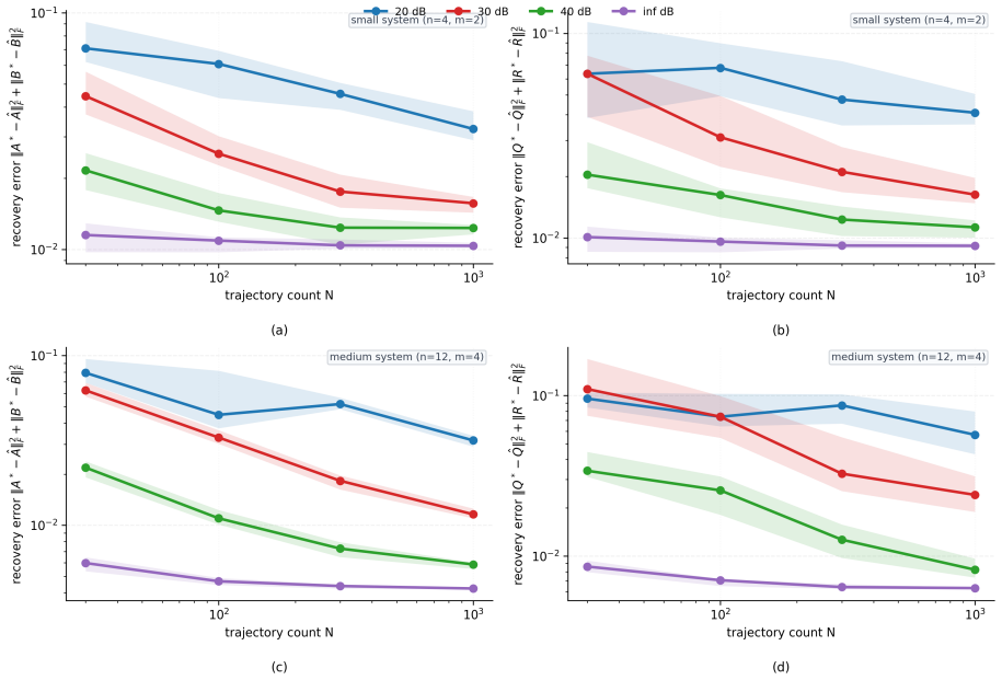
- [Section 6.5, Table 3] The conditioning study reports mean errors over 30 trials but does not provide error bars or quantiles for the three settings; adding them would make the stage-selective degradation in R2 and R3 easier to assess.
Circularity Check
No significant circularity: the identifiability conditions are stated as properties of the true system and gain, not as fitted inputs, and the reconstruction and perturbation analysis are self-contained.
full rationale
The derivation chain is self-contained and does not reduce to its own inputs. Lemma 3.2 recovers the gain K(t) from the algebraic relation U(t) = -K(t)X(t) under full-rank state richness; Theorem 3.3 separates (A,B) from the functional identity A_c(t) = A - B K(t) using the gain-variation Gramian; Theorem 3.7 and Theorem 3.8 concatenate these steps through the stationarity-residual operator M_alpha. The conditions c_AB > 0 and c_QRH > 0 are conditions on the true tuple (A*,B*,Q*,R*,H*) and the induced optimal gain, not parameters fitted to data, and the empirical diagnostics (c_hat_X, c_hat_AB, c_hat_QRH) are used only as computed indicators. The definition of c_QRH as the restricted minimum gain of M_alpha does make Theorem 3.7 a direct reformulation of injectivity, but the paper states this equivalence explicitly and does not present it as an empirical prediction; the cost-recovery SDP, the closed-form dynamics recovery, and the non-asymptotic perturbation bounds contain independent content. Assumption 2.2 (H = alpha Q) is an admitted structural restriction, and Proposition 3.5 explicitly shows non-identifiability outside it, so it is a scope limitation rather than circular reasoning. The unquantified err_ODE term in Lemma 5.9 is a gap in the non-asymptotic guarantee, but it is an external numerical error assumed to vanish and is not a circular reuse of the target result. No load-bearing self-citation chain or ansatz-smuggling is present. The identifiability theory is therefore not circular. 0/10.
Assumptions & free parameters
assumptions (7)
- standard math Standard finite-horizon LQR optimality: the optimal control is unique and has the form u(t) = -K(t)x(t) with K(t) = R^{-1}B^T P(t) and P solving the Riccati differential equation.
- standard math Representation of terminal-value Lyapunov equations via variation of constants (Lemma 2.4).
- standard math Sub-Gaussian concentration inequalities for sums of independent sub-Gaussian vectors (Vershynin, Section 2.5).
- domain assumption Assumptions A1-A3: (A,B) stabilizable, rank(B)=m, and rank(X(0))=n.
- domain assumption Assumption 2.2: H = alpha*Q for a known scalar alpha >= 0.
- domain assumption Assumption 4.1: observation noises are zero-mean, independent, and sub-Gaussian.
- domain assumption Assumption 5.1: boundedness and Lipschitz regularity of trajectories, gain, and closed-loop matrix.
Cite this review
Pith. "Pith review of Joint Identifiability and Conditioning in Finite-Horizon Continuous-Time Inverse LQR with Unknown Dynamics." pith.science (2026). https://pith.science/paper/XL3ZSDCA
@misc{pith2026260811932,
  author       = {Pith},
  title        = {Pith review of: Joint Identifiability and Conditioning in Finite-Horizon Continuous-Time Inverse LQR with Unknown Dynamics},
  year         = {2026},
  howpublished = {\url{https://pith.science/paper/XL3ZSDCA}},
  note         = {Machine review of arXiv:2608.11932}
}
abstract
Inverse Optimal Control (IOC) aims to infer the underlying cost functional of an agent from observations of its expert behavior. This paper studies the finite-horizon continuous-time inverse LQR problem from closed-loop state--input trajectories, where both the system matrices and the quadratic cost are unknown. The finite horizon induces a time-varying optimal gain, and this endogenous excitation serves as the structural mechanism that makes joint recovery possible. We quantify this mechanism through three computable conditioning indices, which measure state richness, gain-variation richness, and injectivity of a structured cost operator. Using these indices, we establish joint identifiability conditions for the inverse problem considered here. Crucially, these conditions guarantee recovery of the ground-truth system matrices $(A,B)$ and the true cost weighting matrices, rather than merely a behaviorally equivalent surrogate. We also develop a conditioning-aware sampled-data reconstruction method that reconstructs the gain $K(\cdot)$ and the closed-loop dynamics matrix $A_c(\cdot)$ from noisy measurements, recovers $(A,B)$ in closed form, and identifies the quadratic weights through a convex semidefinite program. We further establish the non-asymptotic perturbation bounds and the consistency of the full reconstruction method under sub-Gaussian observation noise, with explicit dependence on the same conditioning indices. Numerical experiments support the theory and illustrate the diagnostic value of the conditioning indices.
Figures


Figures from the paper (2 more)


Reference graph
Works this paper leans on
-
[1]
F. L. Lewis, D. Vrabie, and V. L. Syrmos,Optimal control. John Wiley & Sons, 2012
2012
-
[2]
From inverse optimal control to inverse reinforce- ment learning: A historical review,
N. Ab Azar, A. Shahmansoorian, and M. Davoudi, “From inverse optimal control to inverse reinforce- ment learning: A historical review,”Annual Reviews in Control, vol. 50, pp. 119–138, 2020
work page 2020
-
[3]
A survey of inverse reinforcement learning,
S. Adams, T. Cody, and P. A. Beling, “A survey of inverse reinforcement learning,”Artificial Intelligence Review, vol. 55, no. 6, pp. 4307–4346, 2022
2022
-
[4]
Inverse optimization: Theory and applications,
T. C. Chan, R. Mahmood, and I. Y. Zhu, “Inverse optimization: Theory and applications,”Operations Research, vol. 73, no. 2, pp. 1046–1074, 2025
work page 2025
-
[5]
When is a linear control system optimal?
R.E.Kalman, “When is a linear control system optimal?”Journal of Basic Engineering, vol. 86, no. 1, pp. 51–60, 1964
work page 1964
-
[6]
S. Boyd, L. El Ghaoui, E. Feron, and V. Balakrishnan,Linear matrix inequalities in system and control theory. Society for Industrial and Applied Mathematics, 1994
work page 1994
-
[8]
H. Zhang, A. Ringh, W. Jiang, S. Li, and X. Hu, “Statistically consistent inverse optimal control for linear-quadratic tracking with random time horizon,” in2022 41st Chinese Control Conference (CCC), 2022, pp. 1515–1522
work page 2022
-
[9]
Inverse kalman filtering problems for discrete-time systems,
Y. Li, B. Wahlberg, X. Hu, and L. Xie, “Inverse kalman filtering problems for discrete-time systems,” Automatica, vol. 163, p. 111560, 2024
work page 2024
Show all 35 references
-
[10]
Bi-level-based inverse stochastic optimal control,
P. Karg, M. Hess, B. Varga, and S. Hohmann, “Bi-level-based inverse stochastic optimal control,” in 2024 European Control Conference (ECC), 2024, pp. 537–544
2024
-
[11]
Discrete-time inverse optimal control with partial- state information: A soft-optimality approach with constrained state estimation,
T. L. Molloy, D. Tsai, J. J. Ford, and T. Perez, “Discrete-time inverse optimal control with partial- state information: A soft-optimality approach with constrained state estimation,” in2016 IEEE 55th Conference on Decision and Control (CDC), 2016, pp. 1926–1932
2016
-
[12]
Control law learning based on LQR reconstruction with inverse optimal control,
C. Qu, J. He, and X. Duan, “Control law learning based on LQR reconstruction with inverse optimal control,”IEEE Transactions on Automatic Control, vol. 70, no. 2, pp. 1350–1357, 2025
2025
-
[13]
Inverse optimal control problem in the non autonomous linear-quadratic case,
F. Jean and S. Maslovskaya, “Inverse optimal control problem in the non autonomous linear-quadratic case,”arXiv:2406.14270, 2024
2024 arXiv
-
[14]
Inverse linear-quadratic discrete-time finite-horizon optimal control for indis- tinguishable homogeneous agents: A convex optimization approach,
H. Zhang and A. Ringh, “Inverse linear-quadratic discrete-time finite-horizon optimal control for indis- tinguishable homogeneous agents: A convex optimization approach,”Automatica, vol. 148, p. 110758, 2023
2023
-
[15]
Inverse optimal control for passive network systems,
L. Hallinan, J. D. Watson, and I. Lestas, “Inverse optimal control for passive network systems,”IEEE Transactions on Automatic Control, 2025
2025
-
[16]
3DIOC: Direct data-driven inverse optimal control for LTI systems,
C. Qu, J. He, and X. Duan, “3DIOC: Direct data-driven inverse optimal control for LTI systems,” arXiv:2409.10884, 2024
2024 arXiv
-
[17]
Inverse reinforcement Q-learning through expert imitation for discrete-time systems,
W. Xue, B. Lian, J. Fan, P. Kolaric, T. Chai, and F. L. Lewis, “Inverse reinforcement Q-learning through expert imitation for discrete-time systems,”IEEE Transactions on Neural Networks and Learning Sys- tems, vol. 34, no. 5, pp. 2386–2399, 2021
2021
-
[18]
Pontryagin differentiable programming: An end-to-end learning and control framework,
W. Jin, Z. Wang, Z. Yang, and S. Mou, “Pontryagin differentiable programming: An end-to-end learning and control framework,”Advances in Neural Information Processing Systems, vol. 33, pp. 7979–7992, 2020. 37
2020
-
[19]
A differential dynamic programming framework for inverse reinforcement learning,
K. Cao, X. Xu, W. Jin, K. H. Johansson, and L. Xie, “A differential dynamic programming framework for inverse reinforcement learning,”IEEE Transactions on Robotics, 2025
2025
-
[20]
On convex data-driven inverse optimal control for nonlinear, non-stationary and stochastic systems,
E. Garrabe, H. Jesawada, C. Del Vecchio, and G. Russo, “On convex data-driven inverse optimal control for nonlinear, non-stationary and stochastic systems,”Automatica, vol. 173, p. 112015, March 2025
2025
-
[21]
Inferring system and opti- mal control parameters of closed-loop systems from partial observations,
V. Geadah, J. Arbelaiz, H. Ritz, N. D. Daw, J. D. Cohen, and J. W. Pillow, “Inferring system and opti- mal control parameters of closed-loop systems from partial observations,” in2024 IEEE 63rd Conference on Decision and Control (CDC). IEEE, 2024, pp. 8006–8013
2024
-
[22]
Data-driven inverse optimal control for linear quadratic tracking with unknown target states,
R. Cheng, C. Yu, and Y. Li, “Data-driven inverse optimal control for linear quadratic tracking with unknown target states,”Automatica, vol. 185, p. 112822, 2026
2026
-
[23]
The approximate arithmetical solution by finite differences of physical problems involving differential equations, with an application to the stresses in a masonry dam,
L. F. Richardson, “The approximate arithmetical solution by finite differences of physical problems involving differential equations, with an application to the stresses in a masonry dam,”Philosophical Transactions of the Royal Society of London. Series A, vol. 210, no. 459–47...
1911
-
[24]
System identification approach for inverse optimal control of finite-horizon discrete-time LQR,
C. Yu, Z. Gao, and Y. Li, “System identification approach for inverse optimal control of finite-horizon discrete-time LQR,”Automatica, vol. 129, p. 109636, July 2021
2021
-
[25]
Continuous-time inverse quadratic optimal control problem,
Y. Li, Y. Yao, and X. Hu, “Continuous-time inverse quadratic optimal control problem,”Automatica, vol. 117, p. 108977, 2020
2020
-
[26]
Inverse continuous-time linear quadratic regulator: From control cost matrix to entire cost reconstruction,
Y. Cao, Y. Li, Z. Zou, and X. Hu, “Inverse continuous-time linear quadratic regulator: From control cost matrix to entire cost reconstruction,”arXiv:2510.04083, 2025
2025
-
[27]
B. D. O. Anderson and J. B. Moore,Optimal Control: Linear Quadratic Methods. Dover Publications, 2007
2007
-
[28]
Inverse optimal control for discrete-time finite-horizon linear quadratic regulators,
H. Zhang, J. Umenberger, and X. Hu, “Inverse optimal control for discrete-time finite-horizon linear quadratic regulators,”Automatica, vol. 110, p. 108593, 2019
2019
-
[29]
Constrained model predictive control: Stability and optimality,
D. Q. Mayne, J. B. Rawlings, C. V. Rao, and P. O. M. Scokaert, “Constrained model predictive control: Stability and optimality,”Automatica, vol. 36, no. 6, pp. 789–814, 2000
2000
-
[30]
J. B. Rawlings and D. Q. Mayne,Model Predictive Control: Theory and Design. Nob Hill Publishing, 2009
2009
-
[31]
Survey of extrapolation processes in numerical analysis,
D. C. Joyce, “Survey of extrapolation processes in numerical analysis,”SIAM Review, vol. 13, no. 4, pp. 435–490, 1971
1971
-
[32]
Vershynin,High-Dimensional Probability: An Introduction with Applications in Data Science
R. Vershynin,High-Dimensional Probability: An Introduction with Applications in Data Science. Cam- bridge: Cambridge University Press, 2018
2018
-
[33]
On the sample complexity of the linear quadratic regulator,
S. Dean, H. Mania, N. Matni, B. Recht, and S. Tu, “On the sample complexity of the linear quadratic regulator,”Foundations of Computational Mathematics, vol. 20, no. 4, pp. 633–679, 2020
2020
-
[34]
Certainty equivalence is efficient for linear quadratic control,
H. Mania, S. Tu, and B. Recht, “Certainty equivalence is efficient for linear quadratic control,” in Advances in Neural Information Processing Systems, vol. 32, 2019
2019
-
[35]
CVXPY: A python-embedded modeling language for convex optimization,
S. Diamond and S. Boyd, “CVXPY: A python-embedded modeling language for convex optimization,” Journal of Machine Learning Research, vol. 17, no. 83, pp. 1–5, 2016
2016
-
[36]
Clarabel: An interior-point solver for conic programs with quadratic objectives,
P. J. Goulart and Y. Chen, “Clarabel: An interior-point solver for conic programs with quadratic objectives,” 2024. 38
2024
Reviewed August 16, 2026 · model on record in the stance chip above.
Discussion (0). Continue with ORCID to comment.