REVIEW 2 major objections 5 minor 69 references
Accelerating a Strong-Coupling Non-Equilibrium Steady-State Impurity Solver using (Quantics) Tensor Trains
T0 review · 2 major / 5 minor · reviewed 2026-08-15 · deepseek-v4-flash
Pith's one-line read The paper claims that a fused quantics time-difference parametrization with tensor cross interpolation and a direct carry-based QTT retarded convolution reduces the cost of high-order strong-coupling diagrams enough to make…
desk verdict Useful QTT acceleration of strong-coupling NESS impurity solvers, with a real algorithmic contribution; the physical convergence claims are weakened by not extrapolating the eta=0.01 broadening. read the letter →
The pith
A machine-rendered reading of the paper's core claim, the machinery that carries it, and where it could break.
The reading
What carries the argument
The central object is the fused quantics time-difference tensor train of the diagrammatic integrand, together with a direct retarded convolution in the quantics format. A time-difference index is split into binary bits and cores at the same bit level are fused, so the integrand becomes a product of small bit-indexed cores. The time-ordering Heaviside mask has an exact fused QTT representation with bond dimension two. The retarded convolution is implemented as a rank-2 MPO that carries the binary addition $u_r+v_r+\gamma_r = w_r + 2\gamma_{r+1}$ through an auxiliary carry bit $\gamma_r$, which increases the bond dimension by a factor of two, or up to four with trapezoidal endpoint corrections, instead of the roughly eleven-fold growth of a quantics Fourier transform. This object is what converts the nested time-ordered sum into a sequence of small matrix contractions over the bit cores, and it is the component that makes the third-order self-consistent loops fast enough for routine use.
What would settle it
Run the photodoped DMFT and EDMFT calculations at $\eta = 0.01$, $0.02$, $0.04$ and with an annealed $\eta \to 0$ protocol; if the quasiparticle-peak amplitude and Mott-gap edges drift as strongly as the $\eta$-scan in Figure 20, then the TOA-vs-OCA differences could be an artifact of the broadening and the third-order convergence claim is not controlled. A complementary check is to compare the fused-QTT TOA self-energy against a direct quadrature evaluation on a coarser grid where direct evaluation is still feasible.
Extended reading notes
Core claim
The paper's central claim is that the practical limit of nonequilibrium strong-coupling solvers is lifted: by writing each nth-order self-energy diagram in the Keldysh time-difference parametrization, expanding every time-difference index into binary bits, and grouping bits by scale into a fused quantics tensor train via tensor cross interpolation, the expensive time-ordered integral becomes a product of small matrix contractions. The retarded convolutions that enforce time ordering are applied directly within the quantics format through a rank-2 carry-bit transfer operator, avoiding Fourier transforms. The paper argues, and demonstrates on Gaussian benchmarks, that the resulting bond dimensions are independent of grid size and only grow modestly with diagram order, so that self-consistent DMFT iterations at NCA, OCA, and TOA can be run routinely, and the same machinery handles impurity models with retarded density-density interactions inside nonequilibrium EDMFT. Its headline numerical results are that OCA Bethe DMFT iterations take seconds on a laptop and TOA iterations minutes on a 96-core node.
Load-bearing premise
The load-bearing premise is that the pseudo-particle propagators decay within the numerical cutoff $t_c=327.67$, or equivalently that the artificial broadening $\eta=0.01$ used in the main DMFT runs is a controlled approximation to the $\eta \to 0$ limit, so that neither the finite window nor the damping distorts the spectral peaks enough to change the apparent order-by-order convergence.
Editorial extensions
If this is right
- Nonequilibrium DMFT on the Bethe lattice can be iterated self-consistently at NCA, OCA, and TOA, giving controlled order-by-order convergence checks instead of stopping at OCA.
- In the Mott-regime the strong-coupling series converges quickly, while in the correlated metal higher orders are needed; TOA availability directly improves quasiparticle-peak predictions.
- Impurity models with retarded density-density interactions, the core of EDMFT and GW+EDMFT, can now be solved with an error estimate from comparing NCA, OCA, and TOA; the results indicate NCA overestimates Mott-gap stability while OCA and TOA are close.
- With the fused quantics time-difference solver, OCA Bethe DMFT iterations take seconds on a laptop and TOA iterations minutes on a 96-core node.
- The direct QTT convolution algorithm is reusable for other Volterra or convolution-type integral equations, and may eventually allow the entire DMFT self-consistency cycle to run inside the QTT representation.
Reading between the lines
- Because the carry-based convolution is exact at the bit level, the same operation should accelerate the pseudo-particle Dyson-equation step itself; the paper only sketches this as a future possibility.
- The method's crossover depends on the time cutoff: for short simulation windows, the non-quantics time-difference parametrization with higher-order Gregory quadrature can remain faster, so an adaptive choice based on the required $t_c$ and decay rate would be a natural extension.
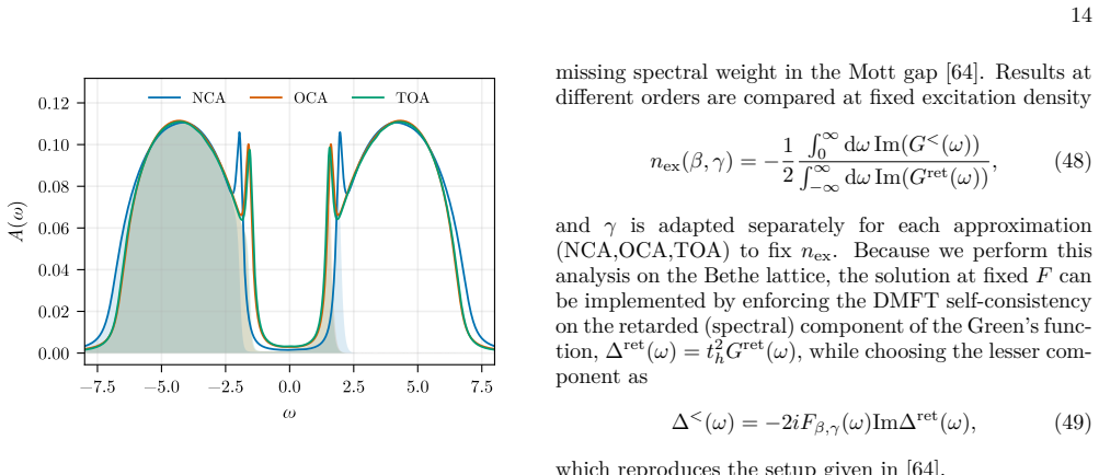
- The $\eta$-dependence shown in the paper's Figure 20 implies that spectral features sharper than roughly $\eta$ may be systematically suppressed; an annealed $\eta \to 0$ procedure, which the paper does not present, is the cleanest way to test whether TOA corrections to the quasiparticle peak remain significant.
- The moderate bond-dimension growth from OCA to TOA in the Gaussian benchmark suggests the same machinery can reach still higher orders before rank growth becomes prohibitive, rather than encountering a topological ceiling.
Signed reviews
Editorial analysis
A structured set of objections, weighed in public.
Referee Report
Summary. The manuscript develops tensor-cross-interpolation (TCI) and quantics tensor-train (QTT) parametrizations for evaluating high-order strong-coupling (hybridization expansion) diagrams for nonequilibrium steady-state impurity solvers. Four parametrizations are compared: absolute-time TCI, quantics absolute-time, time-difference TCI, and quantics time-difference, the last using a newly derived direct carry-bit retarded convolution in fused QTT form. Gaussian benchmarks are used to compare accuracy, bond dimensions, and runtime; the methods are then applied to self-consistent equilibrium DMFT with a fluctuation-dissipation diagnostic, to photodoped nonequilibrium Bethe-lattice DMFT up to third order (TOA), and to square-lattice EDMFT with retarded density-density interactions. The central claim is that the quantics time-difference approach makes OCA and TOA self-consistent iterations practical, enabling controlled order-by-order convergence checks in regimes previously limited to NCA/OCA.
Significance. If the efficiency and accuracy claims hold, this is a substantial methodological advance. The carry-based direct QTT retarded convolution is a reusable algorithmic ingredient, and the demonstration of self-consistent TOA-level nonequilibrium DMFT and EDMFT would open a regime previously inaccessible to systematic strong-coupling expansions. Credit is due for the careful benchmark design: TCI errors are measured against direct quadrature on the same grid, convergence is scanned independently in bond dimension and grid size, and the equilibrium fluctuation-dissipation relation is used as a nontrivial self-consistency check. The main weakness is that the central physical convergence claims are made at a single artificial broadening parameter in the pseudo-particle Dyson equation, with only partial evidence that the results are controlled in that parameter.
major comments (2)
- [Sec. IV C, Fig. 17, App. B, Fig. 20] The central physical conclusion that the TOA results are 'nearly converged' and provide a 'controlled estimate of the truncation error' is established at a single value of the artificial broadening, eta=0.01. Figure 20 shows that for the same photodoped Bethe-lattice parameters the quasiparticle-peak amplitude and position still vary visibly as eta is reduced from 0.04 to 0.01, for NCA, OCA, and TOA alike, and no extrapolation to eta->0 is presented. The text in App. B states that annealing to smaller eta is possible but omits it because the focus is the accelerated solver. This leaves open the possibility that the apparent OCA-TOA closeness in Fig. 17 is partly a broadening artifact rather than genuine order-by-order convergence. Please provide an eta scan for the order-by-order comparison in Fig. 17, or otherwise quantify the eta-induced uncertainty on the claimed truncation error.
- [Sec. V, Fig. 18] The EDMFT results are presented without stating the broadening parameter used or providing an eta-scan, although the bosonic spectra show low-frequency sensitivity and the NCA/OCA/TOA differences are used to claim convergence. The statement that the TOA results are 'already nearly converged' in EDMFT therefore rests on the same unverified broadening assumption as the DMFT results. Please state the value of eta (and the time cutoff) used in Sec. V and provide a convergence check with respect to eta, or explicitly characterize the regime in which the presented results are independent of this parameter.
minor comments (5)
- [Fig. 17 caption and Sec. IV C] The main text says 'eta=0.01 below' in Sec. IV B, but Fig. 17's caption does not state the broadening value; please state the eta used in the caption or in the text immediately preceding the figure.
- [Eq. (47)] The notation Theta_alpha(omega) for the smooth distribution function conflicts with the time-ordering mask Theta_{s1,...,sD} introduced in Eq. (37); please use a different symbol, such as H_alpha(omega) or F_alpha(omega).
- [Sec. IV B and App. B] The statement that the pseudo-particle propagators are 'sufficiently decayed' at t_c=327.67 is asserted for NCA but not quantified. Since eta=0.01 gives a damping scale 1/eta=100 that is active throughout the tail, please report the actual decay of G(t_c) for OCA and TOA, or otherwise provide evidence that the finite-window error is negligible.
- [App. C] The self-convergence test uses the largest available bond dimension chi=160 as the reference, which is reasonable, but the TOA slope is noticeably slower; please state explicitly that this is a self-convergence test and not an absolute error estimate.
- [Sec. VI] The conclusion states that the quantics representation scales as O(log N_t) for sampling; this is logarithmic in N_t only at fixed diagram order and fixed bond dimension, as the complexity is O(2^D R chi^3). Please phrase this more precisely.
Circularity Check
No significant circularity found: the algorithmic claims are benchmarked against independent quadrature and fluctuation-dissipation diagnostics, and no physical result is used to set the method parameters.
full rationale
The paper's central claim is algorithmic: that quantics tensor-train parametrizations with tensor cross interpolation and a direct carry-based QTT retarded convolution reduce the cost of high-order strong-coupling diagrams. This claim is supported by controlled Gaussian benchmarks in Sec. IV A, where the TCI results are compared with direct quadrature on the same grid, and by self-consistent DMFT tests in Sec. IV B where the fluctuation-dissipation relation provides an independent equilibrium diagnostic. The method parameters—bond dimension, grid size, and quadrature weights—are varied and converged without reference to a target physical result, so no fitted parameter is renamed as a prediction. The Keldysh time-difference parametrization is imported from Ref. [55], and the quantics frequency-domain approach from Refs. [56,57], but the paper's new contribution, the direct real-time QTT convolution, is derived in Appendix A and benchmarked independently. The self-citations are to prior technical constructions, and the present performance comparisons are self-contained: the paper compares four parametrizations on the same synthetic integrands and the same DMFT convergence diagnostics. The η-dependence discussed in Sec. II A 3 and Appendix B is a physical-parameter convergence concern, not a circularity: the artificial broadening is not fitted to reproduce the final spectra, and the paper explicitly notes that convergence should be extrapolated to η→0. Likewise, the photodoped OCA-TOA proximity is presented as a truncation-order comparison, not as a predicted quantity that was used to calibrate the solver. Overall, the derivation chain does not contain any step in which an input is defined in terms of an output, nor does the central acceleration claim reduce to a fitted quantity or to an unverified self-citation chain.
Assumptions & free parameters
free parameters (4)
- Maximum bond dimension chi =
varies: 16-192 in Gaussian tests; 15-30 in DMFT
- Time cutoff t_c =
327.67 (DMFT); 8 (Gaussian test)
- Grid size N_t / time step Delta t =
up to 2^17 for QTCI; 2^12 for TCI diff in DMFT
- Artificial broadening eta =
0.01 (main results); 0.005-0.02 considered sensible
assumptions (6)
- domain assumption The strong-coupling (hybridization) expansion for the pseudo-particle self-energy and correlation functions is a valid, systematically improvable diagrammatic series (Eqs. 6-11).
- domain assumption Time-translational invariance holds in the nonequilibrium steady state, so contour functions depend only on time differences (Eq. 12).
- domain assumption Tensor cross interpolation as implemented in the xfac library produces low-rank tensor trains with controlled error for the sampled integrands (Eqs. 19-21).
- standard math The carry-bit transfer MPO exactly implements binary addition for retarded convolutions on the grid without overflow (App. A, Eq. A9).
- domain assumption The artificial pseudo-particle bath with broadening eta and distribution g(omega) provides a controlled regularization whose eta-to-0 limit is physical (App. B).
- domain assumption Self-consistent fixed-point iteration of the Dyson equation converges to the physical solution for the studied parameters.
Cite this review
Pith. "Pith review of Accelerating a Strong-Coupling Non-Equilibrium Steady-State Impurity Solver using (Quantics) Tensor Trains." pith.science (2026). https://pith.science/paper/AWAAU4SX
@misc{pith2026260813146,
  author       = {Pith},
  title        = {Pith review of: Accelerating a Strong-Coupling Non-Equilibrium Steady-State Impurity Solver using (Quantics) Tensor Trains},
  year         = {2026},
  howpublished = {\url{https://pith.science/paper/AWAAU4SX}},
  note         = {Machine review of arXiv:2608.13146}
}
read the original abstract
Including higher order diagrammatic corrections to the strong-coupling expansion is mainly limited by the evaluation of high-dimensional, time-ordered integrals. In this work we present and compare four different parametrizations of the integrands in order to obtain a low-rank (quantics) tensor-train representation using tensor cross interpolation. Particular emphasis is placed on a quantics time-difference formulation in which the required retarded convolutions are performed directly in quantics tensor-train form. Using controlled Gaussian benchmarks, we analyze the accuracy, bond dimensions, and computational scaling of the different approaches. We then validate the most promising formulations in self-consistent equilibrium and nonequilibrium DMFT calculations and demonstrate calculations up to the third order in the strong-coupling expansion. Finally, we extend the solver to impurity models with retarded density-density interactions and apply it within nonequilibrium extended DMFT. Our results show that tensor cross interpolation substantially reduces the cost of evaluating higher-order diagrams and provides a controlled, systematically improvable framework for nonequilibrium quantum impurity calculations.
Figures


Figures from the paper (15 more)




Reference graph
Works this paper leans on
-
[1]
P. W. Anderson, Physical Review124, 41 (1961)
work page 1961
-
[2]
Georges, G
A. Georges, G. Kotliar, W. Krauth, and M. J. Rozenberg, Reviews of Modern Physics68, 13 (1996)
1996
-
[3]
Such states are obtained by taking the initial time to the remote past,t min →−∞
Steady-state formulation In this work, we focus on nonequilibrium steady states (NESS). Such states are obtained by taking the initial time to the remote past,t min →−∞. Assuming that the transient dynamics on the impurity is damped by the coupling to the environment, all correlation functions 4 −∞ C+ C− t2 t1 t3 t0 Figure 1. Steady-state Keldysh contour ...
-
[4]
In a steady state,CAB(t,t′)depends only on time difference
Physical correlation functions From the self-consistent pseudo-particle propagators, physical two-point correlation functions CAB(t,t′) =−i⟨TCA(t)B(t′)⟩(14) must be obtained from a separate diagrammatic expan- sion. In a steady state,CAB(t,t′)depends only on time difference. With the conventional definition of lesser and greater contour-ordered correlatio...
- [5]
-
[6]
Lu and M
Y. Lu and M. W. Haverkort, The European Physical Journal Special Topics226, 2549 (2017)
2017
-
[7]
K. G. Wilson, Reviews of Modern Physics47, 773 (1975)
1975
-
[8]
E. Gull, A. J. Millis, A. I. Lichtenstein, A. N. Rubtsov, M. Troyer, and P. Werner, Rev. Mod. Phys.83, 349 (2011)
2011
Show all 69 references
-
[9]
F. A. Wolf, A. Go, I. P. McCulloch, A. J. Millis, and U. Schollwöck, Phys. Rev. X5, 041032 (2015)
2015
-
[10]
CUI: Advanced Imaging of Matter
is at the minimal error plateau to ensure a fair compari- son. 0 2 4 t 5 0 (t) a) Re > Re < Im > Im < riem trap 64 128 256 5121024 Nt 10 1 (riem) (trap) 2 b) N 1 t Figure 12. Direct Gaussian OCA quadrature comparison be- tween Riemann and trapezoidal integration for a represen...
-
[11]
Bauernfeind, M
D. Bauernfeind, M. Zingl, R. Triebl, M. Aichhorn, and H. G. Evertz, Phys. Rev. X7, 031013 (2017)
2017
-
[12]
Werner, A
P. Werner, A. Comanac, L. de’ Medici, M. Troyer, and A. J. Millis, Physical Review Letters97, 076405 (2006)
2006
-
[13]
A. N. Rubtsov, V. V. Savkin, and A. I. Lichtenstein, Phys. Rev. B72, 035122 (2005)
2005
-
[14]
Mühlbacher and E
L. Mühlbacher and E. Rabani, Phys. Rev. Lett.100, 176403 (2008)
2008
-
[15]
Werner, T
P. Werner, T. Oka, and A. J. Millis, Phys. Rev. B79, 035320 (2009)
2009
-
[16]
Gramsch, K
C. Gramsch, K. Balzer, M. Eckstein, and M. Kollar, Physical Review B88, 235106 (2013)
2013
-
[17]
F. A. Wolf, I. P. McCulloch, and U. Schollwöck, Phys. Rev. B90, 235131 (2014)
2014
-
[18]
Arrigoni, M
E. Arrigoni, M. Knap, and W. Von Der Linden, Physical Review Letters110, 086403 (2013)
2013
-
[19]
R. Chen, X. Xu, and C. Guo, Phys. Rev. B109, 045140 (2024)
2024
-
[20]
Thoenniss, A
J. Thoenniss, A. Lerose, and D. A. Abanin, Phys. Rev. B107, 195101 (2023)
2023
-
[21]
Nayak, J
M. Nayak, J. Thoenniss, M. Sonner, D. A. Abanin, and P. Werner, Phys. Rev. B112, 035103 (2025)
2025
-
[22]
H. Aoki, N. Tsuji, M. Eckstein, M. Kollar, T. Oka, and P. Werner, Reviews of Modern Physics86, 779 (2014)
2014
-
[23]
Murakami, D
Y. Murakami, D. Golež, M. Eckstein, and P. Werner, Rev. Mod. Phys.97, 035001 (2025)
2025
-
[24]
Keiter and J
H. Keiter and J. C. Kimball, Physical Review Letters25, 672 (1970)
1970
-
[25]
Coleman, Physical Review B29, 3035 (1984)
P. Coleman, Physical Review B29, 3035 (1984)
1984
-
[26]
N. E. Bickers, D. L. Cox, and J. W. Wilkins, Phys. Rev. B36, 2036 (1987)
1987
-
[27]
Haule, S
K. Haule, S. Kirchner, J. Kroha, and P. Wölfle, Phys. Rev. B64, 155111 (2001)
2001
-
[28]
A. J. Kim, K. Lenk, J. Li, P. Werner, and M. Eckstein, Phys. Rev. Lett.130, 036901 (2023)
2023
-
[29]
A. J. Kim, J. Li, M. Eckstein, and P. Werner, Phys. Rev. B106, 085124 (2022)
2022
-
[30]
Haule, Strong coupling quantum impurity solver on the real and imaginary axis (2023)
K. Haule, Strong coupling quantum impurity solver on the real and imaginary axis (2023)
2023
-
[31]
J. Kaye, H. U. r. Strand, and N. Wentzell, Journal of Open Source Software9, 6297 (2024)
2024
-
[32]
J. Kaye, K. Chen, and O. Parcollet, Physical Review B 105, 235115 (2022)
2022
-
[33]
Huang, D
Z. Huang, D. Golez, H. U. R. Strand, and J. Kaye, Sci- Post Physics19, 121 (2025)
2025
-
[34]
J. Kaye, Z. Huang, H. U. R. Strand, and D. Golež, Phys- ical Review X14, 031034 (2024)
2024
-
[35]
Eckstein and P
M. Eckstein and P. Werner, Physical Review B82, 115115 (2010)
2010
-
[36]
Eckstein and P
M. Eckstein and P. Werner, Phys. Rev. B84, 035122 (2011)
2011
-
[37]
Cohen, E
G. Cohen, E. Gull, D. R. Reichman, and A. J. Millis, Physical Review Letters115, 266802 (2015)
2015
-
[38]
Erpenbeck, E
A. Erpenbeck, E. Gull, and G. Cohen, Physical Review Letters130, 186301 (2023)
2023
-
[39]
Erpenbeck, T
A. Erpenbeck, T. Blommel, L. Zhang, W.-T. Lin, G. Co- hen, and E. Gull, The Journal of Chemical Physics161, 094104 (2024). 18
2024
-
[40]
D. V. Savostyanov, Linear Algebra and its Applications 458, 217 (2014)
2014
-
[41]
I. V. Oseledets, SIAM Journal on Scientific Computing 33, 2295 (2011)
2011
-
[42]
Oseledets and E
I. Oseledets and E. Tyrtyshnikov, Linear Algebra and its Applications432, 70 (2010)
2010
-
[43]
Núñez Fernández, M
Y. Núñez Fernández, M. Jeannin, P. T. Dumitrescu, T. Kloss, J. Kaye, O. Parcollet, and X. Waintal, Physical Review X12, 041018 (2022)
2022
-
[44]
Dolgov and D
S. Dolgov and D. Savostyanov, Computer Physics Com- munications246, 106869 (2020)
2020
-
[45]
B. N. Khoromskij, Constructive Approximation34, 257 (2011)
2011
-
[46]
Y. N. Fernández, M. K. Ritter, M. Jeannin, J.-W. Li, T. Kloss, T. Louvet, S. Terasaki, O. Parcollet, J. v. Delft, H. Shinaoka, and X. Waintal, SciPost Physics18, 104 (2025), arXiv:2407.02454 [physics]
2025 arXiv
-
[47]
Shinaoka, M
H. Shinaoka, M. Wallerberger, Y. Murakami, K. Nogaki, R. Sakurai, P. Werner, and A. Kauch, Physical Review X13, 021015 (2023)
2023
-
[48]
Frankenbach, M
M. Frankenbach, M. K. Ritter, M. Pelz, N. Ritz, J. Von Delft, and A. Ge, Physical Review Research7, 043032 (2025)
2025
-
[49]
Rohshap, M
S. Rohshap, M. K. Ritter, H. Shinaoka, J. von Delft, M. Wallerberger, and A. Kauch, Physical Review Re- search7, 023087 (2025)
2025
-
[50]
Murray, H
M. Murray, H. Shinaoka, and P. Werner, Physical Review B109, 165135 (2024)
2024
-
[51]
Środa, K
M. Środa, K. Inayoshi, H. Shinaoka, and P. Werner, Physical Review Letters135, 226501 (2025)
2025
-
[52]
Erpenbeck, W.-T
A. Erpenbeck, W.-T. Lin, T. Blommel, L. Zhang, S. Iskakov, L. Bernheimer, Y. Núñez-Fernández, G. Co- hen, O. Parcollet, X. Waintal, and E. Gull, Physical Re- view B107, 245135 (2023)
2023
-
[53]
S.Matsuura, H.Shinaoka, P.Werner,andN.Tsuji,Phys- ical Review B111, 155150 (2025)
2025
-
[54]
Matsuura, H
S. Matsuura, H. Shinaoka, P. Werner, and N. Tsuji, Weak-coupling tensor cross interpolation impurity solver for nonequilibrium dynamical mean-field theory (2026), arXiv:2607.00702 [cond-mat.str-el]
2026 arXiv
-
[55]
Li and M
J. Li and M. Eckstein, Physical Review B103, 045133 (2021), arXiv:2007.12511 [cond-mat]
2021 arXiv
-
[56]
J. Li, D. Golez, P. Werner, and M. Eckstein, Phys. Rev. B102, 165136 (2020)
2020
-
[57]
S. Ray, Y. Murakami, and P. Werner, Phys. Rev. B108, 174515 (2023)
2023
-
[58]
Eckstein, Solving quantum impurity models in the non-equilibrium steady state with tensor trains (2024), arXiv:2410.19707 [cond-mat]
M. Eckstein, Solving quantum impurity models in the non-equilibrium steady state with tensor trains (2024), arXiv:2410.19707 [cond-mat]
2024 arXiv
-
[59]
A. J. Kim and P. Werner, Physical Review B111, 125120 (2025)
2025
-
[60]
L. Geng, A. J. Kim, and P. Werner, Physical Review B 112, 245119 (2025)
2025
-
[61]
Golez, M
D. Golez, M. Eckstein, and P. Werner, Physical Review B92, 195123 (2015), arXiv:1507.07953 [cond-mat]
2015 arXiv
-
[62]
Golež, L
D. Golež, L. Boehnke, H. U. R. Strand, M. Eckstein, and P. Werner, Phys. Rev. Lett.118, 246402 (2017)
2017
-
[63]
Werner and M
P. Werner and M. Eckstein, Physical Review B88, 165108 (2013)
2013
-
[64]
Paprotzki and M
E. Paprotzki and M. Eckstein, Physical Review B112, 205126 (2025)
2025
-
[65]
H.-T. Chen, G. Cohen, A. J. Millis, and D. R. Reichman, Physical Review B93, 174309 (2016)
2016
-
[66]
Kamenev, Field theory of non-equilibrium systems (2023), iSBN: 9781108769266 9781108488259
A. Kamenev, Field theory of non-equilibrium systems (2023), iSBN: 9781108769266 9781108488259
2023
-
[67]
Künzel, A
F. Künzel, A. Erpenbeck, D. Werner, E. Arrigoni, E. Gull, G. Cohen, and M. Eckstein, Physical Review Letters132, 176501 (2024)
2024
-
[68]
Golež, M
D. Golež, M. Eckstein, and P. Werner, Physical Review B100, 235117 (2019)
2019
-
[69]
Inayoshi, H
K. Inayoshi, H. Shinaoka, and Y. Murakami, Generalized keldysh formalism for nonequilibrium correlation func- tions and its application to fluctuation dynamics (2026), arXiv:2607.11055 [cond-mat.str-el]. Appendix A: Retarded Convolution using Quantics Within this section we di...
2026 arXiv
Reviewed August 15, 2026 · model on record in the stance chip above.
Discussion (0). Continue with ORCID to comment.