Making complex CFTs real: The two-dimensional Potts model for Q>4 and complex Q
Pith reviewed 2026-06-26 22:11 UTC · model grok-4.3
The pith
The Potts model for Q>4 yields complex CFTs whose data continue analytically from the Q≤4 loop model.
A machine-rendered reading of the paper's core claim, the machinery that carries it, and where it could break.
Core claim
By studying an equivalent loop model derived from a Potts model with two- and three-spin interactions on the triangular lattice, the authors demonstrate that a critical and a tricritical fixed point collide at Q=4 and then continue as a pair of complex conformally invariant theories for Q>4 or complex Q. They conjecture that the central charge, critical exponents, and three-point structure constants are all obtained by analytic continuation from the Q ≤ 4 case, supported by transfer-matrix computations.
What carries the argument
The loop model with continuously variable Q, obtained from the triangular-lattice Potts model with two- and three-spin interactions, which permits complex couplings that produce a pair of complex fixed points for Q>4.
If this is right
- All conformal data for the Potts model at real Q>4 are given by the analytic continuation of the known Q≤4 loop-model results.
- The same continuation supplies the data when Q itself is taken to be complex.
- The resulting theories remain conformally invariant even though the couplings are complex.
- The numerical spectra obtained by transfer matrix for Q=5 agree with the continued formulas, confirming the pattern.
Where Pith is reading between the lines
- The same continuation technique may apply to other lattice models whose real-coupling versions exhibit first-order transitions.
- Transfer-matrix or Monte Carlo methods could be used to test analytic continuations in related statistical-mechanics models with tunable parameters.
- The construction supplies a concrete route to defining conformal field theories at parameter values where conventional real couplings produce no critical point.
Load-bearing premise
The triangular-lattice Potts model with two- and three-spin interactions remains equivalent to the loop model when Q is continued to values greater than 4 or into the complex plane, provided the couplings are allowed to become complex.
What would settle it
Transfer-matrix computations at some real Q>4 or complex Q that produce central charges or exponents differing from the values predicted by analytic continuation of the Q≤4 formulas would falsify the conjecture.
Figures


read the original abstract
The two-dimensional $Q$-state Potts model with real couplings has a first-order transition for $Q>4$. Starting from a triangular-lattice Potts model with two- and three-spin interactions, we study an equivalent loop model in which $Q$ is a continuous parameter. By a combination of analytical and numerical arguments, we show that this loop model allows for the collision of a critical and a tricritical fixed point at $Q=4$. These then emerge as a pair of complex conformally invariant theories at $Q>4$, or even complex $Q$, for suitable complex coupling constants. We conjecture that all conformal data (such as the central charge, critical exponents, and three-point structure constants) can be obtained by analytic continuation of known exact results for the loop model with $Q \le 4$. This conjecture is checked, both for real $Q>4$ and for $Q \in \mathbb{C}$, by extensive transfer-matrix computations and comparison to previous studies for $Q=5$.
Editorial analysis
A structured set of objections, weighed in public.
Referee Report
Summary. The manuscript conjectures that all conformal data (central charge, critical exponents, three-point structure constants) of the two-dimensional Potts model for real Q>4 or complex Q can be obtained by analytic continuation of known exact loop-model results at Q≤4. Starting from a triangular-lattice Potts model with two- and three-spin interactions, the authors argue analytically that a critical and tricritical fixed point collide at Q=4 and then emerge as a complex-conjugate pair for Q>4 (or complex Q) at suitable complex couplings; they support the conjecture with extensive transfer-matrix spectra that match the continued formulas, including checks against prior Q=5 results.
Significance. If the central conjecture holds, the work supplies a concrete route to conformal data for a family of complex CFTs realized by the Potts model, extending the exactly solvable regime beyond Q=4 while preserving the loop-model interpretation. The combination of fixed-point collision analysis and direct numerical verification of multiple independent quantities (spectra, exponents, structure constants) constitutes a non-trivial test; the provision of reproducible transfer-matrix data and explicit comparisons to existing Q=5 literature are positive features.
major comments (2)
- [§2] §2 (model definition) and the paragraph following Eq. (loop weight): the claim that the Potts-to-loop mapping survives analytic continuation to complex Q and complex couplings is asserted without a re-derivation or explicit check that no new singularities or redefinitions of the loop fugacity appear; this assumption is load-bearing for equating the continued CFT data to the triangular-lattice model.
- [§4.3] §4.3 (transfer-matrix spectra for complex Q): while the numerical eigenvalues are reported to agree with the continued formulas, the manuscript does not quantify the distance to the nearest non-continued singularity or demonstrate that the complex-coupling fixed point remains isolated; without this, the numerical support for the conjecture remains partial.
minor comments (2)
- [Figure 3] Figure 3 caption: the legend does not specify the lattice size used for the Q=5 comparison; adding this datum would improve reproducibility.
- [§2, §3.2] Notation: the symbol for the three-spin coupling is introduced in §2 but reused with a different normalization in §3.2; a single consistent definition would remove ambiguity.
Simulated Author's Rebuttal
We thank the referee for the careful reading and constructive comments. We address the two major comments point by point below, proposing revisions where they strengthen the manuscript without altering its core claims.
read point-by-point responses
-
Referee: §2 (model definition) and the paragraph following Eq. (loop weight): the claim that the Potts-to-loop mapping survives analytic continuation to complex Q and complex couplings is asserted without a re-derivation or explicit check that no new singularities or redefinitions of the loop fugacity appear; this assumption is load-bearing for equating the continued CFT data to the triangular-lattice model.
Authors: The Fortuin-Kasteleyn representation rewrites the Potts partition function as a sum over loop configurations whose weight is exactly Q per loop (up to normalization), and this algebraic identity holds for arbitrary complex values of the two- and three-spin couplings because it follows from expanding the local Boltzmann factors without reference to their magnitude or phase. Consequently the loop fugacity remains Q and no additional singularities are introduced by the mapping itself. We nevertheless agree that an explicit statement improves clarity. We will add a short paragraph in §2 that re-derives the loop weight for complex parameters and confirms the absence of redefinitions. revision: yes
-
Referee: §4.3 (transfer-matrix spectra for complex Q): while the numerical eigenvalues are reported to agree with the continued formulas, the manuscript does not quantify the distance to the nearest non-continued singularity or demonstrate that the complex-coupling fixed point remains isolated; without this, the numerical support for the conjecture remains partial.
Authors: We concur that a quantitative estimate of the distance to the nearest extraneous singularity would strengthen the numerical case. With transfer-matrix spectra on finite strips, however, systematically locating the closest singularity in the multi-dimensional complex-coupling space is not practicable. We have instead verified agreement for several independent observables (eigenvalues, scaling dimensions, and structure constants) at multiple distinct complex-Q and coupling values; the consistency across these checks provides indirect evidence that the fixed point remains isolated within the explored region. We will insert a paragraph in §4.3 that discusses this robustness while explicitly noting the limitation on quantifying isolation. revision: partial
Circularity Check
No significant circularity: conjecture rests on independent exact results plus external numerical checks
full rationale
The paper conjectures that conformal data for Q>4 or complex Q follows by analytic continuation of known exact loop-model results at Q≤4. This continuation is checked by transfer-matrix spectra that constitute an independent numerical test rather than a fit to the same quantities. The Potts-to-loop equivalence for complex parameters is presented as an assumption supported by fixed-point collision arguments at Q=4, but no step reduces by construction to a self-definition, a fitted input renamed as prediction, or a load-bearing self-citation chain. The derivation therefore remains self-contained against external benchmarks.
Axiom & Free-Parameter Ledger
axioms (1)
- domain assumption The triangular-lattice Potts model with two- and three-spin interactions is equivalent to the loop model for continuous real or complex Q.
Reference graph
Works this paper leans on
-
[1]
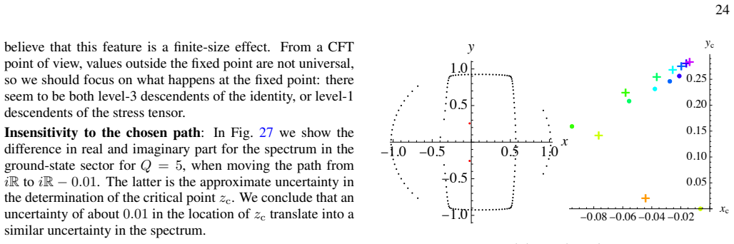
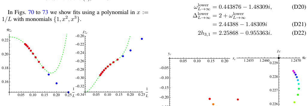
69 to 73) repeats the analysis for the lower half plane
shows the analysis in the upper half plane, while section D 3 (Figs. 69 to 73) repeats the analysis for the lower half plane. This analysis confirms that theory and transfer matrix give the same value forcwith 4-digits accuracy atL= 15, see Eqs. (D14) and (D19). Another key claim of ours is that in contrast toQ= 5, the Potts model at complexQ= 5 + 2ihas b...
-
[2]
Degenerate operatorsV d (r,1) We now study the spectrum atQ= 5in the ground-state sector, using the quotient representation W0,q2 of defect-free FIG. 28. Real and imaginary part∆ (S) r,s of spectrum in the ground- state sector forQ= 5,L= 12, maximally 20 EVs, two consecutive layers. Primaries in dot-dashed, descendents dotted. The dashed vertical lines de...
-
[3]
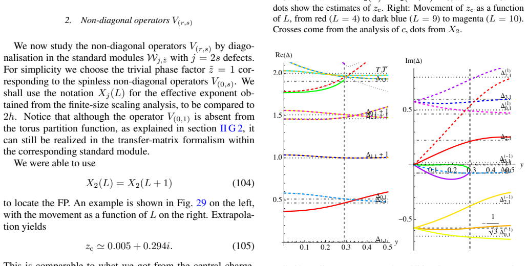
For simplicity we choose the trivial phase factor˜z= 1cor- responding to the spinless non-diagonal operatorsV (0,s)
Non-diagonal operatorsV (r,s) We now study the non-diagonal operatorsV (r,s) by diago- nalisation in the standard modulesW j,˜zwithj= 2sdefects. For simplicity we choose the trivial phase factor˜z= 1cor- responding to the spinless non-diagonal operatorsV (0,s). We shall use the notationX j(L)for the effective exponent ob- tained from the finite-size scali...
-
[4]
From the point of link patterns this means that we now work in a larger space that distin- guishes whether the link between two sites straddles the peri- odic boundary condition
Additional states in the non-quotient spectrum Rather than diagonalizingT L in the quotient representa- tion W0,q2, as in section VII C 1, we also examined the non- quotient representationW 0,q2. From the point of link patterns this means that we now work in a larger space that distin- guishes whether the link between two sites straddles the peri- odic bo...
-
[5]
The dots show the the successive approximations fromc ′(z) = 0
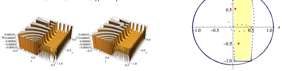
The contour plot shows|∆−1−i/ √ 3|2. The dots show the the successive approximations fromc ′(z) = 0. with conformal weights(1,0), that satisfy ¯∂J=∂ ¯J̸= 0.(111) and which donotgiving rise to a Kac-Moody algebra. Using here our numerical approach atQ= 5, we find at the critical point, indicated with a red dashed line forL= 12in Fig. 31 ∆ = 1.00047 + 0.575...
-
[6]
The result is zc = 0.00182±0.30206i.(113) This should be compared to our best estimate fromc ′(z) = 0, namelyz c = 0.0049 + 0.3007i, see Fig. 20. We finally note that we found another element in the spec- trum, with∆≈2×(1 +i/ √ 3). It can be identified with the stress tensorTwith conformal weights(h, ¯h) = (2,0)
-
[7]
When one is not exactly at the fixed point, there are corrections due to subdominant operators
OPE coefficients: Quotient spectrum corrected byε ′ Up to now we read off exponents as∆ = ∆(z c). When one is not exactly at the fixed point, there are corrections due to subdominant operators. The leading one isε ′ =V d (3,1), in- tegrated over all of space. Denoting bygits effective coupling constant, we expect to see a corrected value∆ corr i,1 (z)[72]...
-
[8]
52.c,L= 10, raw data
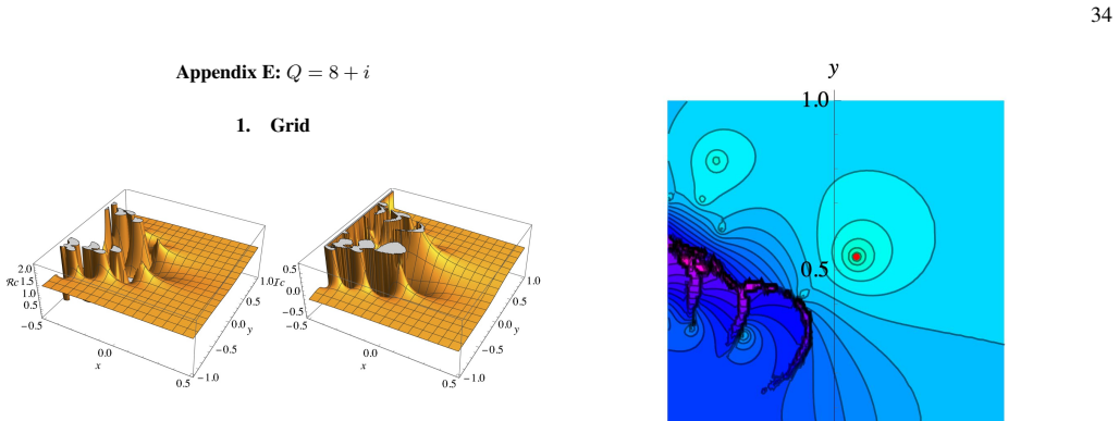
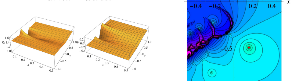
Grid FIG. 52.c,L= 10, raw data. FIG. 53.c,L= 10, selected data. FIG. 54.c,L= 10, subtracted data, upper half plane. FIG. 55.c,L= 10, subtracted data, lower half plane. The contour plot 56 gives a good idea about the location of the singularities. Note that the two non-trivial fixed points marked by the red dots in Fig. 56 are not complex conjugate of each...
-
[9]
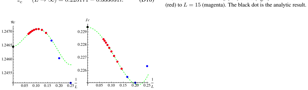
Minigrid, upper half plane Here we use a minigrid of5×5points, centered around the non-trivial fixed point identified in the preceding section. In Fig. 64 we show the area covered by it, as well as the zeroes of the fitting polynomial, for our largest system sizes,L= 15. The non-trivial solution marked in red is clearly visible. -0.4 -0.2 0.2 0.4 x -0.6 -...
-
[10]
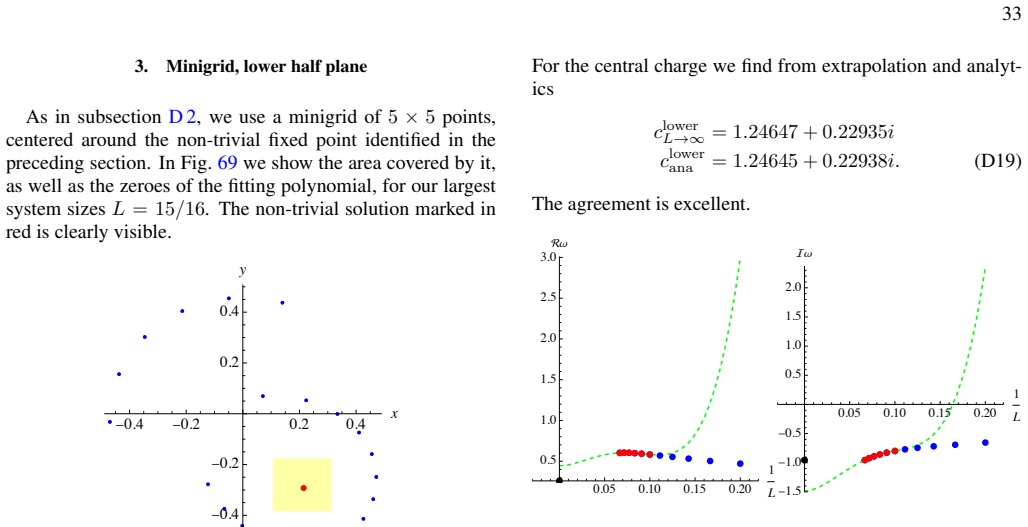
Minigrid, lower half plane As in subsection D 2, we use a minigrid of5×5points, centered around the non-trivial fixed point identified in the preceding section. In Fig. 69 we show the area covered by it, as well as the zeroes of the fitting polynomial, for our largest system sizesL= 15/16. The non-trivial solution marked in red is clearly visible. -0.4 -0...
-
[11]
74.catL= 10, raw data
Grid FIG. 74.catL= 10, raw data. FIG. 75.catL= 10, selected data. FIG. 76.c,L= 10, subtracted, upper half plane. FIG. 77.c,L= 10, subtracted, lower half plane. The contour plot 78 gives a good idea about the location of the singularities. Note that the two non-trivial fixed points marked by the red dots in Fig. 78 are not complex conjugate of each other. ...
-
[12]
As in subsection D 2, we use a minigrid of5×5points, centered around the non-trivial fixed point identified in the preceding section
Minigrid, upper half-plane Again we use a minigrid of5×5points. As in subsection D 2, we use a minigrid of5×5points, centered around the non-trivial fixed point identified in the preceding section. In Fig. 86 we show the area covered by it, as well as the zeroes of the fitting polynomial, for our largest system sizesL= 15. The non-trivial solution marked ...
-
[13]
-0.6 -0.4 -0.2 0.2 0.4 x -0.6 -0.4 -0.2 0.2 0.4 0.6 y FIG
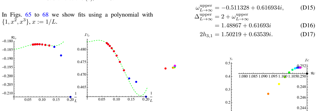
Minigrid, lower half plane Here we use a minigrid of5×5points. -0.6 -0.4 -0.2 0.2 0.4 x -0.6 -0.4 -0.2 0.2 0.4 0.6 y FIG. 91. Zeros ofc ′(z),L= 15, LHP. FixpointB −b Fits for upper half plane. If not stated otherwise, the fitting polynomial contains{1, x 2, x3}, withx:= 1/L. 0.05 0.10 0.15 0.20 0.25 1 L0.08 0.10 0.12 0.14 0.16 ℛzc 0.05 0.10 0.15 0.20 0.25...
-
[14]
Their Eqs
General formulas We follow Dotsenko and Fateev (DF) [84]. Their Eqs. (6) and (7) read in our conventions hn,n′ = 1 4 h (α−n′ +α +n)2 −(α + +α −)2 i ,(G1) c= 1−24α 2 0,(G2) α± =α 0 ± q 1 +α 2 0,(G3) 1 =α +α−.(G4) Comparing to our formulas implies that 4α2 0b(b−1) = 1.(G5) Let us suppose we consider the series of minimal models with b >1, then the appropria...
-
[15]
Due to Eq
Examples of OPE coefficients following DF, physical branch We now give some examples for the formulas in section G. Due to Eq. (G15),2l=s+n−p+ 1as well as2l ′ = 9 Attention, there is a misprint in DF in the first product in the first line after Eq (18). 40 s′ +n ′ −p ′ + 1need to be even. For integer indices this implies that within each group{s, n, p}and...
-
[16]
They are relevant for other models; some of them appear in [14]
Examples of OPE coefficients following DF, non-physical branch Below are OPE coefficients for operators not realized in the Potts model. They are relevant for other models; some of them appear in [14]. Note that this list contains some OPE coeffi- cients with non-integer entries, see Eqs. (G32)-(G33). To compare to the perturbative expansion of [14], we a...
-
[17]
Lee and C.N
T.D. Lee and C.N. Yang,Statistical theory of equations of state and phase transitions. II. Lattice gas and Ising model, Phys. Rev.87(1952) 410–419. 42
1952
-
[18]
Fisher,The nature of critical points, in W
M.E. Fisher,The nature of critical points, in W. E. Brittin, editor,Lecture Notes in Theoretical Physics, V olume7c, pages 1–159, University of Colorado Press, 1965
1965
-
[19]
Salas and A.D
J. Salas and A.D. Sokal,Transfer matrices and partition- function zeros for antiferromagnetic Potts models. I. General theory and square-lattice chromatic polynomial, J. Stat. Phys. 104(2001) 609–699
2001
-
[20]
Fortuin and P.W
C.M. Fortuin and P.W. Kasteleyn,On the random-cluster model: I. Introduction and relation to other models, Physica 57(1972) 536–564
1972
-
[21]
Schramm,Scaling limits of loop-erased random walks and uniform spanning trees, Israel J
O. Schramm,Scaling limits of loop-erased random walks and uniform spanning trees, Israel J. Math.118(2000) 221–288, arXiv:math/9904022
Pith/arXiv arXiv 2000
-
[22]
Sheffield,Exploration trees and conformal loop ensembles, Duke Math
S. Sheffield,Exploration trees and conformal loop ensembles, Duke Math. J.147(2009) 79–129, math/0609167
Pith/arXiv arXiv 2009
-
[23]
Rohde and O
S. Rohde and O. Schramm,Basic properties of SLE, pages 989–1030, Springer, New York, NY , 2011
2011
-
[24]
Baxter,Potts model at the critical temperature, J
R.J. Baxter,Potts model at the critical temperature, J. Phys. C 6(1973) L445
1973
-
[25]
K.J. Wiese and J.L. Jacobsen,The two upper critical dimen- sions of the Ising and Potts models, JHEP05(2024) 092, arXiv:2311.01529
arXiv 2024
-
[26]
Ma and Y .-C
H. Ma and Y .-C. He,Shadow of complex fixed point: Approx- imate conformality ofQ >4Potts model, Phys. Rev. B99 (2019) 195130
2019
-
[27]
Cardy, M
J.L. Cardy, M. Nauenberg and D.J. Scalapino,Scaling theory of the Potts-model multicritical point, Phys. Rev. B22(1980) 2560–2568
1980
-
[28]
C. Wang, A. Nahum, M.A. Metlitski, C. Xu and T. Senthil, Deconfined quantum critical points: Symmetries and dualities, Phys. Rev. X7(2017) 031051
2017
-
[29]
Nahum,Fixed point annihilation for a spin in a fluctuating field, Phys
A. Nahum,Fixed point annihilation for a spin in a fluctuating field, Phys. Rev. B106(2022) L081109
2022
-
[30]
Gorbenko, S
V . Gorbenko, S. Rychkov and B. Zan,Walking, Weak first- order transitions, and Complex CFTs II. Two-dimensional Potts model atQ >4, SciPost Phys.5(2018) 50
2018
-
[31]
Nienhuis,Exact critical point and critical exponents ofO(n) models in two dimensions, Phys
B. Nienhuis,Exact critical point and critical exponents ofO(n) models in two dimensions, Phys. Rev. Lett.49(1982) 1062– 1065
1982
-
[32]
Haldar, O
A. Haldar, O. Tavakol, H. Ma and T. Scaffidi,Hidden critical points in the two-dimensionalO(n >2)model: Exact numeri- cal study of a complex conformal field theory, Phys. Rev. Lett. 131(2023) 131601
2023
-
[33]
Guo, H.W.J
W. Guo, H.W.J. Bl ¨ote and F.Y . Wu,Phase transition in the n >2honeycombO(n)model, Phys. Rev. Lett.85(2000) 3874–3877
2000
-
[34]
J.L. Jacobsen and K.J. Wiese,Lattice realization of complex CFTs: Two-dimensional Potts model withQ >4states, Phys. Rev. Lett.133(2024) 077101, arXiv:2402.10732
arXiv 2024
-
[35]
Y . Tang, H. Ma, Q. Tang, Y .-C. He and W. Zhu,Reclaiming the lost conformality in a non-hermitian quantum 5-state Potts model, Phys. Rev. Lett.133(2024) 076504, arXiv:2403.00852
arXiv 2024
-
[36]
Y . Tang, Q. Liu, Q. Tang and W. Zhu,Boundary criticality of complex conformal field theory: A case study in the non- Hermitian 5-state Potts model, SciPost Phys.19(2025) 164
2025
-
[37]
H.N.V . Temperley and E.H Lieb,Relations between the ‘per- colation’ and ‘colouring’ problem and other graph-theoretical problems associated with regular planar lattices: some exact results for the ‘percolation’ problem, Proc. Roy. Soc. A (1971)
1971
-
[38]
Wu and K.Y
F.Y . Wu and K.Y . Lin,On the triangular Potts model with two- and three-site interactions, J. Phys. A13(1980) 629
1980
-
[39]
Baxter, H.N.V
R.J. Baxter, H.N.V . Temperley and S.E. Ashley,Triangular Potts model at its transition temperature, and related models, Proc. R. Soc. Lond. A358(1978) 535–559
1978
-
[40]
Baxter, S.B
R.J. Baxter, S.B. Kelland and F.Y . Wu,Equivalence of the Potts model or Whitney polynomial with an ice-type model, J. Phys. A9(1976) 397
1976
-
[41]
Nienhuis,Critical behaviour of two-dimensional spin mod- els and charge asymmetry in the Coulomb gas, J
B. Nienhuis,Critical behaviour of two-dimensional spin mod- els and charge asymmetry in the Coulomb gas, J. Stat. Phys.34 (1984) 731–61
1984
-
[42]
Belavin, A.M
A.A. Belavin, A.M. Polyakov and A.B. Zamolodchikov,Infinite conformal symmetry in two-dimensional quantum field theory, Nucl. Phys. B241(1984) 333–380
1984
-
[43]
Di Francesco, H
P. Di Francesco, H. Saleur and J.B. Zuber,Relations between the Coulomb gas picture and conformal invariance of two- dimensional critical models, J. Stat. Phys.49(1987) 57–79
1987
-
[44]
J.L. Jacobsen, S. Ribault and H. Saleur,Spaces of states of the two-dimensionalO(n)and Potts models, SciPost Phys.14 (2023) 092, arXiv:2208.14298
arXiv 2023
-
[45]
R. Nivesvivat, S. Ribault and J.L. Jacobsen,Critical loop models are exactly solvable, SciPost Phys.17(2024) 029, arXiv:2311.17558
arXiv 2024
-
[46]
Kondev,Liouville field theory of fluctuating loops, Phys
J. Kondev,Liouville field theory of fluctuating loops, Phys. Rev. Lett.78(1997) 4320
1997
-
[47]
Cardy,SLE for theoretical physicists, Ann
J. Cardy,SLE for theoretical physicists, Ann. Phys. (NY)318 (2005) 81–118, cond-mat/0503313v2
Pith/arXiv arXiv 2005
-
[48]
Lawler,Conformally Invariant Processes in the Plane, V olume114ofMathematical Surveys and Monographs, Amer- ican Mathematical Society, 2005
G.F. Lawler,Conformally Invariant Processes in the Plane, V olume114ofMathematical Surveys and Monographs, Amer- ican Mathematical Society, 2005
2005
-
[49]
Lawler,Schramm-Loewner evolution, (2007), arXiv:0712.3256
G.F. Lawler,Schramm-Loewner evolution, (2007), arXiv:0712.3256
Pith/arXiv arXiv 2007
-
[50]
Guillarmou, R
C. Guillarmou, R. Rhodes and V . Vargas,Polyakov’s formu- lation of 2d bosonic string theory, Publ. Math. Inst. Hautes Etudes Sci.130(2019) 111–185
2019
-
[51]
Guillarmou, A
C. Guillarmou, A. Kupiainen, R. Rhodes and V . Vargas,Con- formal bootstrap in Liouville theory, Acta Math.233(2024) 33–194
2024
-
[52]
Dorn and H.-J
H. Dorn and H.-J. Otto,Two- and three-point functions in Li- ouville theory, Nucl. Phys. B429(1994) 375–388
1994
-
[53]
Zamolodchikov and A.l
A. Zamolodchikov and A.l. Zamolodchikov,Conformal boot- strap in Liouville field theory, Nucl. Phys. B477(1996) 577– 605
1996
-
[54]
M. Picco, R. Santachiara, J. Viti and G. Delfino,Connectivities of Potts Fortuin-Kasteleyn clusters and time-like Liouville cor- relator, Nucl. Phys. B875(2013) 719–737, arXiv:1304.6511
Pith/arXiv arXiv 2013
-
[55]
Ikhlef, J.L
Y . Ikhlef, J.L. Jacobsen and H. Saleur,Three-point functions in c≤1Liouville theory and conformal loop ensembles, Phys. Rev. Lett.116(2016) 130601
2016
-
[56]
Zamolodchikov,Three-point function in the minimal Li- ouville gravity, Theor
A.B. Zamolodchikov,Three-point function in the minimal Li- ouville gravity, Theor. Math. Phys.142(2005) 183–196, hep- th/0505063
arXiv 2005
-
[57]
M. Ang, G. Cai, X. Sun and B. Wu,SLE loop measure and Liouville quantum gravity2024, arXiv:2409.16547
-
[59]
Y . He, J.L. Jacobsen and H. Saleur,Geometrical four-point functions in the two-dimensional criticalQ-state Potts model: The interchiral conformal bootstrap, JHEP2020(2020) 19, arXiv: 2005.07258
arXiv 2020
-
[60]
L. Grans-Samuelsson, J.L. Jacobsen, R. Nivesvivat, S. Rib- ault and H. Saleur,From combinatorial maps to correla- tion functions in loop models, SciPost Phys.15(2023) 147, arXiv:2302.08168
arXiv 2023
-
[61]
P. Roux, J.L. Jacobsen, R. Nivesvivat and S. Ribault, Three-point functions in critical loop models, (2025), arXiv:2510.04701
Pith/arXiv arXiv 2025
-
[62]
Roux, J.L
P. Roux, J.L. Jacobsen, S. Ribault and H. Saleur,Critical spin chains and loop models withP SU(n)symmetry, SciPost Phys. 43 18(2025) 033
2025
-
[63]
Jacobsen, J
J.L. Jacobsen, J. Salas and C.R Scullard,Phase diagram of the triangular-lattice Potts antiferromagnet, J. Phys. A50(2017) 345002
2017
-
[64]
Jacobsen and H
J.L. Jacobsen and H. Saleur,The antiferromagnetic transition for the square-lattice Potts model, Nucl. Phys. B743(2006) 207–248
2006
-
[65]
Baxter,Critical antiferromagnetic square-lattice Potts model, Proc
R.J. Baxter,Critical antiferromagnetic square-lattice Potts model, Proc. R. Soc. A383(1982) 43
1982
-
[66]
Ikhlef, J
Y . Ikhlef, J. Jacobsen and H. Saleur,A staggered six-vertex model with non-compact continuum limit, Nucl. Phys. B789 (2008) 483–524
2008
-
[67]
Ikhlef, J.L
Y . Ikhlef, J.L. Jacobsen and H. Saleur,Integrable spin chain for theSL(2, r)/U(1)black hole sigma model, Phys. Rev. Lett. 108(2012) 081601
2012
-
[68]
Bazhanov,Extended Z-invariance for integrable vector and face models and multi-component integrable quad equa- tions, J
V .V . Bazhanov,Extended Z-invariance for integrable vector and face models and multi-component integrable quad equa- tions, J. Stat. Phys.176(2019) 1375–1408
2019
-
[69]
Di Francesco, P
P. Di Francesco, P. Mathieu and D. S ´en´echal,Conformal Field Theory, Springer, New York, 1997
1997
-
[70]
A. B. Zamolodchikov,Renormalization group and perturbation theory near fixed points in two-dimensional field theory, Yad. Fiz.46(1987) 1819–1831, Sov. J. Nucl. Phys. 46 (1987) 1090– 1096
1987
-
[71]
B ¨ohm, Y
J. B ¨ohm, Y . Jacobsen, J.L.and Jiang and Y . Zhang,Geomet- ric algebra and algebraic geometry of loop and Potts models, JHEP2022(2022) 68
2022
-
[72]
Jacobsen and H
J.L. Jacobsen and H. Saleur,Bootstrap approach to geometri- cal four-point functions in the two-dimensional criticalQ-state Potts model: a study of the s-channel spectra, JHEP2019 (2019) 84
2019
-
[73]
R. Couvreur, J.L. Jacobsen and R. Vasseur,Non-scalar opera- tors for the Potts model in arbitrary dimension, J. Phys. A50 (2017) 474001, arXiv:1704.02186
Pith/arXiv arXiv 2017
-
[74]
Dotsenko and V .A
Vl.S. Dotsenko and V .A. Fateev,Conformal algebra and multi- point correlation functions in 2d statistical models, Nucl. Phys. B240(1984) 312 – 348
1984
-
[75]
Roux,BarnesDoubleGamma.jl: Julia package for comput- ing the Barnes Double Gamma and Double Sine functions in arbitrary precision,2024
P. Roux,BarnesDoubleGamma.jl: Julia package for comput- ing the Barnes Double Gamma and Double Sine functions in arbitrary precision,2024
2024
-
[76]
Y . Tang, H. Ma, Q. Tang, Y .-C. He and W. Zhu, private com- munication
-
[77]
Itzykson, R.B
C. Itzykson, R.B. Pearson and J.B. Zuber,Distribution of zeros in Ising and gauge models, Nucl. Phys. B220(1983) 415–433
1983
-
[78]
Chen, C.-K Hu and F.Y
C.-N. Chen, C.-K Hu and F.Y . Wu,Partition function zeros of the square lattice Potts model, Phys. Rev. Lett.76(1996) 169– 172
1996
-
[79]
Kim,Fisher zeros of the Ising antiferromagnet in an ar- bitrary nonzero magnetic field, Phys
S.-Y . Kim,Fisher zeros of the Ising antiferromagnet in an ar- bitrary nonzero magnetic field, Phys. Rev. E71(2005) 017102
2005
-
[80]
Chang, J
S.C. Chang, J. Salas and R. Shrock,Exact Potts model parti- tion functions for strips of the square lattice, J. Stat. Phys.107 (2002) 1207–1253
2002
-
[81]
Buffenoir and S
E. Buffenoir and S. Wallon,The correlation length of the Potts model at the first-order transition point, J. Phys. A26(1993) 3045
1993
discussion (0)
Sign in with ORCID, Apple, or X to comment. Anyone can read and Pith papers without signing in.