REVIEW 2 major objections 4 minor 136 references
The scaling limit of planar maps with large faces
T0 review · 2 major / 4 minor · reviewed 2026-08-09 · deepseek-v4-flash
Pith's one-line read The paper constructs, for each α∈(1,2), a universal random compact metric space S_α — the α-stable carpet in the dilute phase and α-stable gasket in the dense phase — and proves that all non-generic critical Boltzmann planar maps of…
desk verdict A very strong paper: explicit stable limits for non-generic Boltzmann maps, with the re-rooting reduction in Section 7.4.2 as the main unverified link. read the letter →
The pith
A machine-rendered reading of the paper's core claim, the machinery that carries it, and where it could break.
The reading
What carries the argument
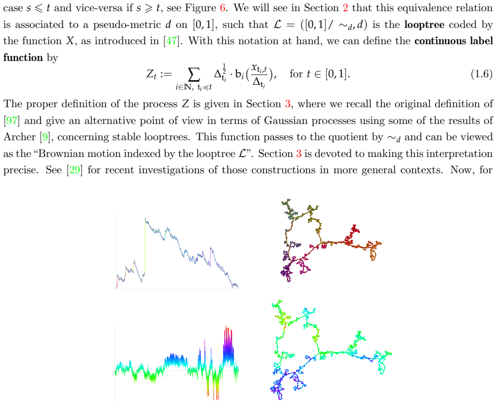
The load-bearing objects are the α-stable looptree L coded by a spectrally positive α-stable Lévy excursion (loops glued along jumps), and the label process Z, defined as the Gaussian process on L with covariance given by the resistance metric — equivalently, Brownian motion indexed by the looptree. The proof works by (1) encoding discrete maps by labeled trees via a classical labeled-tree bijection, (2) passing to the coding-process limit (X,Z), (3) using fine properties of Z — absence of one-sided records on the skeleton, density of records on loops, and the exact two-point function — to prove that every subsequential limit identifies exactly the same points as the explicit pseudo-distance D*, and (4) a two-source labeled-tree construction to control geodesics between typical points and a surgery argument showing D and D* agree.
What would settle it
Take two non-generic weight sequences with the same α and simulate large conditioned Boltzmann maps; compute the rescaled Gromov–Hausdorff–Prokhorov limits (for example via distance matrices between a growing cloud of sampled vertices) and the Hausdorff dimension of the limiting space. If the two limits differ or the dimension is not 2α, Theorem 1.1 is false. A smaller-scale check: evaluate N(sup Z>1) by Monte Carlo on a discretized stable looptree with independent Brownian bridges on each loop; the paper's two-point function identities imply the exact value α(α−1)/2, so any discrepancy would trace the failure to the continuum construction.
Extended reading notes
Core claim
The central discovery is that the scaling limit of non-generic critical Boltzmann maps with exponent α exists and is described explicitly by a stable Lévy excursion X decorated by a Gaussian label process Z, the Brownian motion indexed by the stable looptree. The limiting space S_α is [0,1]/∼_{D*} with D* built from Z; the argument shows every subsequential limit D equals D* by identifying which points are glued — only trivial identifications in the looptree or zero-distance — and by showing geodesics between typical points are unique and can be compared via a two-source construction. En route the paper establishes fine quantitative facts: local minima of Z avoid the skeleton of the looptree; the two-point function satisfies N(sup Z>1)=α(α−1)/2; the volume of root-centered balls has stretched-exponential tails; geodesics to the root are simple, the cut locus is totally disconnected, and the maximal number of geodesics from a point is 2.
Load-bearing premise
The proof depends on the non-genericity condition (1.2), which requires the root-face degree tail to be asymptotic to a specific constant times $k^{{-α}}$ and to involve the same s_q appearing in the rescaling; if that fine-tuned condition fails, the limit is not claimed to be S_α.
Editorial extensions
If this is right
- Every non-generic critical Boltzmann map with exponent α belongs to a single universality class: its scaling limit is S_α, independent of all other details of the face-weight sequence q.
- The Hausdorff dimension 2α of S_α gives a new exact exponent for distances in these maps, refining the earlier tightness exponent.
- The dichotomy at α=3/2 is sharp: for α∈[3/2,2) the limit is almost surely homeomorphic to the Sierpinski carpet, while for α∈(1,3/2) its faces touch, so the topology changes at the dilute/dense transition.
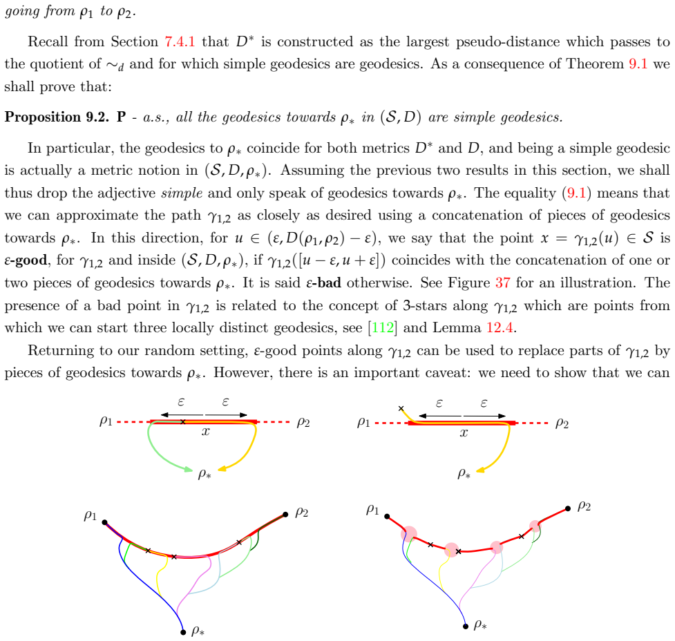
- In any such limit, the geodesics toward a typical root point are simple, the cut locus is totally disconnected, and at most two distinct geodesics can start from the same point.
- The volume of balls in S_α has stretched-exponential tail bounds, providing a robust local estimate usable in further metric-geometric analysis.
Reading between the lines
- Not proved in the paper: the same convergence should hold if the non-genericity hypothesis is weakened to regular variation or if bipartiteness is dropped; the paper only sketches a re-rooting route toward these extensions.
- Not proved in the paper: if the conjectural link to γ-LQG is correct, S_α should coincide with the chemical metric inside a conformal loop ensemble, giving these spaces a conformal-geometric characterization.
- Not proved in the paper: as α→2, the construction should degenerate to the Brownian-sphere regime, interpolating between the stable and Brownian universality classes.
- Not proved in the paper: the exact value N(sup Z>1)=α(α−1)/2 yields an explicit candidate for the two-point distance distribution, testable by simulation of the continuum process or of large maps.
Editorial analysis
A structured set of objections, weighed in public.
Referee Report
Summary. The paper constructs, for each alpha in (1,2), a random compact metric measure space (S_alpha, D*_alpha, Vol_alpha) from a normalized alpha-stable Levy excursion decorated by independent Brownian bridges, and claims that large critical non-generic Boltzmann bipartite planar maps with weight sequence q of exponent alpha converge in distribution to this space after scaling distances by (s_q n)^{-1/(2 alpha)}. The claimed limit is universal, depending on q only through alpha, and has Hausdorff dimension 2 alpha. The introduction describes a proof strategy: tightness from [97]; identification of the point equivalence via faces; uniqueness of geodesics via a two-source construction; surgery along geodesics; and a priori ball-volume estimates. The paper also proves that in the dilute phase alpha in [3/2,2) the limit is homeomorphic to the Sierpinski carpet, while in the dense phase alpha in (1,3/2) faces may touch.
Significance. If Theorem 1.1 holds, this is a major advance: it establishes the first universal scaling limits for non-generic Boltzmann maps with large faces, constructs the stable carpets/gaskets, and develops a rich continuum theory (Gaussian free field on looptrees, exact two-point function, geodesic classification). The paper is notable for the exact computation N(sup Z > 1) = alpha(alpha-1)/2 via Bessel and hypergeometric functions, for the spinal decomposition of the label process, and for the topology theorems, including the Sierpinski carpet statement in the dilute phase. The introduction is exemplary in outlining a long and intricate proof. Credible strengths include the detailed treatment of the coding process and the robust a priori estimates leading to a dimension bound. The main caveat is that the proof of full Theorem 1.1 relies on deferred re-rooting and surgery arguments that are not verified in the material under review.
major comments (2)
- [Section 1 (after (1.5)); Section 7.4.2] Theorem 1.1 is stated for every admissible, critical, non-generic weight sequence q satisfying the tail condition (1.2). The text after (1.5) says that the proof is first carried out under the stronger pointwise condition w_q(deg(root face)=k) ~ C k^{-alpha-1}, and that the full statement follows from Le Gall's re-rooting trick, with details deferred to Section 7.4.2. Section 7.4.2 is not included in the material under review. This reduction is load-bearing: it must preserve the universal limiting space S_alpha and the normalization (s_q n)^{-1/(2 alpha)} for every q satisfying the fine-tuned condition (1.2). If the re-rooting argument requires additional regularity or yields a q-dependent limit or a different scaling constant, then Theorem 1.1 as stated is not established. Please provide the full details of Section 7.4.2, or restrict the statement of Theorem 1.1 to the pointwise condition and present the extension to the tail condition (1.2) as a conditional result.
- [Proof of Theorem 1.1; Sections 8-12] The introduction states that the equality D = D* for every subsequential limit is proven via the identification of equivalence classes (Theorem 8.1), the two-point construction with delays (Sections 10-11), the uniqueness of the typical geodesic (Theorem 9.1), and the surgery argument with bad-point estimates (Proposition 9.3 and Section 12). These sections are only summarized heuristically in the introduction and are not part of the reviewed text. Since these are the core steps that go beyond [97] and establish the uniqueness of the subsequential limit, the central claim of Theorem 1.1 cannot be fully verified from the supplied material. This is a structural verification gap rather than an identified mathematical error, and the authors should ensure that the complete proof is available in the version under review.
minor comments (4)
- [Index of notation] The entry for PMroot contains duplicated 'of' and a typo: 'isometry classes of of (rooted) iweighted geodesic compact metric spaces' should read 'isometry classes of (rooted) weighted geodesic compact metric spaces'.
- [Section 3.2, proof of Proposition 3.3] In several displays, the symbols 'eδ' and 'ed' are used where '~δ' and '~d' are intended (e.g., in the computation of the Brownian bridge covariance and in the final display of the proof). Please correct these typographical errors.
- [Section 5.2, proof of Proposition 5.4] The vanishing of the constants A' and B' in the hypergeometric expansion is asserted with 'a (tedious) computation shows that A'=B'=0', but the computation is not provided. Since the resulting value alpha(alpha-1)/2 determines the phase transition at alpha=3/2 and feeds into Proposition 5.6, please include the calculation in an appendix or give a precise reference.
- [Theorem 1.1 statement] The term 'admissible' in 'admissible, critical and non-generic weight sequence' is not defined in the introduction; please give a definition or a reference at the point of first use.
Circularity Check
No significant circularity: the paper's central contribution is the independent proof of uniqueness of subsequential limits, D = D*, built on prior external work rather than on its own conclusions.
full rationale
The derivation chain is incremental and non-circular. The maps are encoded by labeled mobiles via the Bouttier–Di Francesco–Guitter bijection; the scaling limit (X, Z) of these coding trees and the resulting tightness of the rescaled metric spaces are imported from Le Gall and Miermont [97]. That is a prior published result with stated assumptions that do not include Theorem 1.1, so it is legitimate external support even though one of the present authors is a co-author of [97]. The genuinely load-bearing new content is the proof that every subsequential limit metric D equals the explicitly constructed pseudo-distance D*: this is done through the point-identification theorem (Theorem 8.1), the two-point geodesic construction, uniqueness of typical geodesics, the strict upper bound on the dimension of bad points, and the surgery argument along geodesics. None of these steps is defined in terms of the target limit, and no fitted parameter is renamed as a prediction. The limit space S_alpha is built from the same stable excursion and Brownian bridges that appear in the coding-tree limit, but this is the standard structural route for Brownian-type scaling limits and does not make the conclusion equivalent to its inputs. The paper explicitly records that the non-genericity condition (1.2) is fine-tuned and that the reduction from the pointwise asymptotic to the tail condition via the re-rooting trick is deferred to Section 7.4.2; this is an omitted-proof/completeness concern about the full generality of Theorem 1.1, not a circularity. The computation of the constant alpha(alpha-1)/2 and the two-point function are self-contained continuum calculations. Overall, no circular step is identifiable in the reviewed material.
Assumptions & free parameters
assumptions (3)
- domain assumption The weight sequence q is non-generic with exponent alpha in (1,2), i.e. w_q(deg(root face) > k) ~ 2 s_q / |Gamma(1-alpha)| k^{-alpha} (eq. 1.2).
- domain assumption All maps are bipartite, so faces have even degree and the BDG bijection applies.
- standard math The coding functions of the labeled mobiles converge to (X,Z), the stable excursion and the label process, as established in Le Gall and Miermont [97].
Cite this review
Pith. "Pith review of The scaling limit of planar maps with large faces." pith.science (2026). https://pith.science/paper/2UOKE4P2
@misc{pith2026250118566,
  author       = {Pith},
  title        = {Pith review of: The scaling limit of planar maps with large faces},
  year         = {2026},
  howpublished = {\url{https://pith.science/paper/2UOKE4P2}},
  note         = {Machine review of arXiv:2501.18566}
}
abstract
We prove that large Boltzmann stable planar maps of index $\alpha \in (1;2)$ converge in the scaling limit towards a random compact metric space $\mathcal{S}_{\alpha}$ that we construct explicitly. They form a one-parameter family of random continuous spaces ``with holes'' or ``faces'' different from the Brownian sphere. In the so-called dilute phase $\alpha \in [3/2;2)$, the topology of $\mathcal{S}_{\alpha}$ is that of the Sierpinski carpet, while in the dense phase $\alpha \in (1;3/2)$ the ``faces'' of $\mathcal{S}_{\alpha}$ may touch each-others. En route, we prove various geometric properties of these objects concerning their faces or the behavior of geodesics.
Figures


Figures from the paper (44 more)










Reference graph
Works this paper leans on
-
[97]
J.-F. Le Gall and G. Miermont. Scaling limits of random planar maps with large faces. Ann. Probab., 39(1):1–69, 2011
work page 2011
-
[1]
Abraham, J.-F
R. Abraham, J.-F. Delmas, and P. Hoscheit. A note on the Gromov-Hausdorff-Prokhorov dis- tance between (locally) compact metric measure spaces. Electron. J. Probab., 18, 2013
2013
-
[2]
Conditioning (sub)critical L{\'e}vy trees by their maximal degree: Decomposition and local limit
R. Abraham, J.-F. Delmas, and M. Nassif. Conditioning (sub)critical L´ evy trees by their maximal degree: Decomposition and local limit. arXiv:2211.02317, 2022
work page Pith review arXiv 2022
-
[3]
Addario-Berry and M
L. Addario-Berry and M. Albenque. The scaling limit of random simple triangulations and random simple quadrangulations. Ann. Probab., 45(5):2767–2825, 2017
2017
-
[4]
Geometric properties of spin clusters in random triangulations coupled with an Ising Model
M. Albenque and L. M´ enard. Geometric properties of spin clusters in random triangulations coupled with an Ising model. arXiv:2201.11922, 2022. 178
work page Pith review arXiv 2022
-
[5]
Ambjørn, T
J. Ambjørn, T. Budd, and Y. Makeenko. Generalized multicritical one-matrix models. Nuclear Physics B , 913:357–380, 2016
2016
-
[6]
Ambrosio, J
V. Ambrosio, J. Miller, and Y. Yuan. Chemical distance metric for non-simple CLE. (in preparation), 2024
2024
-
[7]
G. E. Andrews, R. Askey, and R. Roy. Special Functions, volume 71 of Cambridge Studies in Advanced Mathematics. Cambridge University Press, Cambridge, 1999
1999
Show all 136 references
-
[8]
Angel, B
O. Angel, B. Kolesnik, and G. Miermont. Stability of geodesics in the Brownian map. Ann. Probab., 45(5):3451–3479, 2017
2017
-
[9]
E. Archer. Brownian motion on stable looptrees. In Annales de l’Institut Henri Poincar´ e- Probabilit´ es et Statistiques, volume 57, pages 940–979, 2021
2021
-
[10]
Archer, A
E. Archer, A. Carrance, and L. M´ enard. Some properties of stable snakes. arXiv:2403.15275, 2024
2024 arXiv
-
[11]
Archer, A
E. Archer, A. Carrance, and L. M´ enard. Stable quadrangulations and stable spheres. arXiv:2405.05677, 2024
2024 arXiv
-
[12]
E. W. Barnes. The genesis of the double Gamma function. Proceedings of the London Mathe- matical Society, 31:358–381, 1899
-
[13]
E. W. Barnes. The theory of the double Gamma function. Philosophical Transactions of the Royal Society of London (A) , 196:265–387, 1901
1901
-
[14]
Berestycki
N. Berestycki. Diffusion in planar Liouville quantum gravity. Ann. Inst. Henri Poincar´ e Probab. Stat., 51(3):947–964, 2015
2015
-
[15]
Bernardi, N
O. Bernardi, N. Curien, and G. Miermont. A Boltzmann approach to percolation on random triangulations. Canadian Journal of Mathematics , 71(1):1–43, 2019
2019
-
[16]
J. Bertoin. Increase of stable processes. J. Theoret. Probab., 7(3):551–563, 1994
1994
-
[17]
J. Bertoin. L´ evy processes, volume 121 of Cambridge Tracts in Mathematics . Cambridge Uni- versity Press, Cambridge, 1996
1996
-
[18]
J. Bertoin. Subordinators: examples and applications. In Lectures on probability theory and statistics (Saint-Flour, 1997) , volume 1717 of Lecture Notes in Math. , pages 1–91. Springer, Berlin, 1999
1997
-
[19]
Bertoin, T
J. Bertoin, T. Budd, N. Curien, and I. Kortchemski. Martingales in self-similar growth- fragmentations and their connections with random planar maps. Probab. Theory Related Fields, 172(3):663–724, 2018. 179
2018
-
[20]
Bertoin, N
J. Bertoin, N. Curien, and A. Riera. Self-similar markov trees and scaling limits. arXiv:2407.07888, 2024
2024 arXiv
-
[21]
Bertoin and M
J. Bertoin and M. Savov. Some applications of duality for L´ evy processes in a half-line. Bulletin of the London Mathematical Society , 43(1):97–110, 10 2010
2010
-
[22]
Bettinelli
J. Bettinelli. Scaling limit of random planar quadrangulations with a boundary. In Annales de l’IHP Probabilit´ es et statistiques, volume 51, pages 432–477, 2015
2015
-
[23]
Bettinelli
J. Bettinelli. Geodesics in Brownian surfaces (Brownian maps). Ann. Inst. Henri Poincar´ e Probab. Stat., 52(2):612–646, 2016
2016
-
[24]
Bettinelli, E
J. Bettinelli, E. Jacob, and G. Miermont. The scaling limit of uniform random plane maps, via the Ambjørn-Budd bijection. Electronic J. Probab., 19, 2014
2014
-
[25]
Bettinelli and G
J. Bettinelli and G. Miermont. Compact Brownian surfaces I: Brownian disks. Probab. Theory Related Fields, 167(3-4):555–614, 2017
2017
-
[26]
Bettinelli and G
J. Bettinelli and G. Miermont. Compact Brownian surfaces II. Orientable surfaces. arXiv:2212.12511, 2022
2022
-
[27]
Bj ¨ornberg, N
J. Bj ¨ornberg, N. Curien, and S. ¨O. Stef´ ansson. Stable shredded spheres and causal random maps with large faces. Ann. of Probab., 50(5):2056–2084, 2022
2022
-
[28]
Blanc, N
G. Blanc, N. Curien, and J. Kahn. Geodesics in planar Poisson roads random metric. arXiv:2407.07887, 2024
2024 arXiv
-
[29]
Blanc-Renaudie
A. Blanc-Renaudie. Looptree, Fennec, and Snake of ICRT. arXiv:2203.10891, 2022
2022 arXiv
-
[30]
Borot, J
G. Borot, J. Bouttier, and E. Guitter. Loop models on random maps via nested loops: case of domain symmetry breaking and application to the potts model. J. Phys. A: Math. Theor. , 45(49), 2012
2012
-
[31]
Borot, J
G. Borot, J. Bouttier, and E. Guitter. A recursive approach to the O(N) model on random maps via nested loops. J. Phys. A: Math. Theor. , 45, 2012
2012
-
[32]
Bouttier, P
J. Bouttier, P. Di Francesco, and E. Guitter. Planar maps as labeled mobiles. Electron. J. Combin., 11(1):Research Paper 69, 27 pp. (electronic), 2004
2004
-
[33]
Bouttier, E
J. Bouttier, E. Guitter, and G. Miermont. Bijective enumeration of planar bipartite maps with three tight boundaries, or how to slice pairs of pants. Annales Henri Lebesgue , 5:1035–1110, 2022
2022
-
[34]
Bretagnolle
J. Bretagnolle. Sur l’in´ egalit´ e de concentration de Doeblin-L´ evy, Rogozin-Kesten. InParametric and semiparametric models with applications to reliability, survival analysis, and quality of life , Stat. Ind. Technol., pages 533–551. Birkh ¨auser Boston, Boston, MA, 2004. 180
2004
-
[35]
Budd and L
T. Budd and L. Chen. The peeling process on random planar maps coupled to an O(n) loop model (with an appendix by Linxiao Chen). Electron. J. Probab., 2019
2019
-
[36]
Budd and N
T. Budd and N. Curien. Geometry of infinite planar maps with high degrees. Electron. J. Probab., 22:Paper No. 35, 37, 2017
2017
-
[37]
Budd and N
T. Budd and N. Curien. Random punctured hyperbolic surfaces & the Brownian sphere. (in preparation), 2024
2024
-
[38]
T. Budd, N. Curien, and C. Marzouk. Infinite random planar maps related to Cauchy processes. J. ´Ec. polytech. Math., 5:749–791, 2018
2018
-
[39]
Burago, Y
D. Burago, Y. Burago, and S. Ivanov. A course in metric geometry , volume 33 of Graduate Studies in Mathematics . American Mathematical Society, Providence, RI, 2001
2001
-
[40]
Caraceni and N
A. Caraceni and N. Curien. Self-avoiding walks on the UIPQ. In Sojourns in Probability Theory and Statistical Physics-III , pages 138–165. Springer, 2019
2019
-
[41]
Chassaing and G
P. Chassaing and G. Schaeffer. Random planar lattices and integrated superBrownian excursion. Probab. Theory Related Fields, 128(2):161–212, 2004
2004
-
[42]
Chaumont
L. Chaumont. Conditionings and path decompositions for L´ evy processes. Stochastic Process. Appl., 64(1):39–54, 1996
1996
-
[43]
Chaumont and G
L. Chaumont and G. Uribe Bravo. Shifting processes with cyclically exchangeable increments at random. XI Symposium on Probability and Stochastic Processes , (69):101–117, 2015
2015
-
[44]
Chen and J
L. Chen and J. Turunen. Critical ising model on random triangulations of the disk: enumeration and local limits. Communications in Mathematical Physics , 374(3):1577–1643, 2020
2020
-
[45]
Chen and J
L. Chen and J. Turunen. Ising model on random triangulations of the disk: phase transition. Communications in Mathematical Physics , 397(2):793–873, 2023
2023
-
[46]
N. Curien. Peeling Random Planar Maps: ´Ecole d’ ´Et´ e de Probabilit´ es de Saint-Flour XLIX– 2019, volume 2335. Springer Nature, 2023
2019
-
[47]
Curien and I
N. Curien and I. Kortchemski. Random stable looptrees. Electron. J. Probab., 19:no. 108, 35, 2014
2014
-
[48]
Curien and J.-F
N. Curien and J.-F. Le Gall. Random recursive triangulations of the disk via fragmentation theory. Ann. Probab., 39(6):2224–2270, 2011
2011
-
[49]
Curien and J.-F
N. Curien and J.-F. Le Gall. The Brownian plane. J. Theoret. Probab., 27(4):1249–1291, 2014
2014
-
[50]
Curien and J.-F
N. Curien and J.-F. Le Gall. First-passage percolation and local perturbations on random planar maps. Ann. Sci. ´Ec. Norm. Sup´ er, 3(52):631–701, 2019. 181
2019
-
[51]
Curien, J.-F
N. Curien, J.-F. Le Gall, and G. Miermont. The Brownian cactus I. Scaling limits of discrete cactuses. Ann. Inst. Henri Poincar´ e Probab. Stat., 49(2):340–373, 2013
2013
-
[52]
Curien, L
N. Curien, L. M´ enard, and G. Miermont. A view from infinity of the uniform infinite planar quadrangulation. ALEA Lat. Am. J. Probab. Math. Stat. , 10(1):45–88, 2013
2013
-
[53]
Curien and L
N. Curien and L. Richier. Duality of random planar maps via percolation. InAnnales de l’Institut Fourier, volume 70, pages 2425–2471, 2020
2020
-
[54]
Dauvergne
D. Dauvergne. The 27 geodesic networks in the directed landscape. arXiv:2302.07802, 2023
2023 arXiv
-
[55]
J.-F. Delmas. Computation of moments for the length of the onedimensional ISE support. Electron. J. Probab., 8:1–15, 2003
2003
-
[56]
Doherty, K
C. Doherty, K. Kavvadias, and J. Miller. Connectivity of the adjacency graph of complementary components of the SLE fan. arXiv:2411.13133, 2024
2024 arXiv
-
[57]
Duplantier, J
B. Duplantier, J. R. Miller, and S. Sheffield. Liouville quantum gravity as a mating of trees. Asterisque, 427, 2021
2021
-
[58]
Duquesne
T. Duquesne. A limit theorem for the contour process of conditioned Galton-Watson trees. Ann. Probab., 31(2):996–1027, 2003
2003
-
[59]
Duquesne and J.-F
T. Duquesne and J.-F. Le Gall. Random trees, L´ evy processes and spatial branching processes. Ast´ erisque, (281):vi+147, 2002
2002
-
[60]
Duquesne and J.-F
T. Duquesne and J.-F. Le Gall. Probabilistic and fractal aspects of L´ evy trees. Probab. Theory Related Fields, 131(4):553–603, 2005
2005
-
[61]
P. J. Fitzsimmons, B. Fristedt, and L. A. Shepp. The set of real numbers left uncovered by random covering intervals. Z. Wahrsch. Verw. Gebiete , 70(2):175–189, 1985
1985
-
[62]
Garban, R
C. Garban, R. Rhodes, and V. Vargas. Liouville Brownian motion. Ann. of Probab., 44(4):3076– 3110, 2016
2016
-
[63]
R. K. Getoor. Excursions of a Markov Process. Ann. of Probab., 7(2):244 – 266, 1979
1979
-
[64]
Topological characterization of the Sierpinski curve
G.Whyburn. Topological characterization of the Sierpinski curve. Fund. Math. 45 , 1958
1958
-
[65]
E. Gwynne. Geodesic networks in Liouville quantum gravity surfaces. Probab. Math. Phys. , 2(3):643–684, 2021
2021
-
[66]
Gwynne, N
E. Gwynne, N. Holden, and X. Sun. Mating of trees for random planar maps and Liouville quantum gravity: a survey. arXiv:1910.04713, 2019
1910 arXiv
-
[67]
Gwynne and J
E. Gwynne and J. Miller. Convergence of percolation on uniform quadrangulations with bound- ary to SLE 6 on √ 8/3-Liouville quantum gravity. arXiv:1701.05175, 2017. 182
2017 arXiv
-
[68]
Gwynne and J
E. Gwynne and J. Miller. Existence and uniqueness of the Liouville quantum gravity metric for γ ∈ (0, 2). Invent. Math., pages 1–121, 2020
2020
-
[69]
Gwynne and J
E. Gwynne and J. Miller. Convergence of the self-avoiding walk on random quadrangulations to SLE8/3 on √ 8/3-Liouville quantum gravity. Ann. Sci. ´Ec. Norm. Sup´ er., 54:305–405, 2021
2021
-
[70]
Gwynne, J
E. Gwynne, J. Miller, and S. Sheffield. The Tutte embedding of the mated-CRT map converges to Liouville quantum gravity. Ann. Probab., 49(4):1677–1717, 2021
2021
-
[71]
Gwynne and J
E. Gwynne and J. Pfeffer. Connectivity properties of the adjacency graph of SLE κ bubbles for κ ∈ (4, 8). Ann. of Probab., 48(3):1495–1519, 2020
2020
-
[72]
J. Hawkes. Intersections of markov random sets. Zeitschrift f ¨ur Wahrscheinlichkeitstheorie und Verwandte Gebiete, 37(3):243–251, 1977
1977
-
[73]
I. A. Ibragimov and Y. V. Linnik. Independent and stationary sequences of random variables . Wolters-Noordhoff Publishing, Groningen, 1971. With a supplementary chapter by I. A. Ibrag- imov and V. V. Petrov, Translation from the Russian edited by J. F. C. Kingman
1971
-
[74]
Kammerer
E. Kammerer. Scaling limit of first passage percolation geodesics on planar maps. arXiv:2412.02666
-
[75]
Kammerer
E. Kammerer. Distances on the CLE4, critical Liouville quantum gravity and 3/2-stable maps. arXiv:2311.08571, 2024
2024
-
[76]
Kammerer
E. Kammerer. Gaskets of O(2) loop-decorated random planar maps. arXiv:2411.05541, 2024
2024
-
[77]
Kammerer
E. Kammerer. On large 3/2-stable maps. Annales de l’Institut Henri Poincar´ e, To appear
-
[78]
R. Khanfir. Convergences of looptrees coded by excursions. Annales de l’Institut Henri Poincar´ e, To appear
-
[79]
A. Khezeli. Metrization of the Gromov–Hausdorff (-Prokhorov) topology for boundedly-compact metric spaces. Stochastic Processes and their Applications , 130(6):101–117, 2020
2020
-
[80]
A. Khezeli. A unified framework for generalizing the Gromov-Hausdorff metric. Probability Surveys, 20:837–896, 2023
2023
-
[81]
Kortchemski
I. Kortchemski. Random stable laminations of the disk. Ann. of Probab., 42(2):725–759, 2014
2014
-
[82]
Kortchemski and C
I. Kortchemski and C. Marzouk. Random L´ evy Looptrees and L´ evy maps. arXiv:2402.04098, 2024
2024 arXiv
-
[83]
Kuratowski
K. Kuratowski. Topology II. Academic Press, New York, (1968)
1968
-
[84]
Kuznetsov
A. Kuznetsov. On extrema of stable processes. Ann. of Probab., 39:1027–1060, 2011. 183
2011
-
[85]
A. E. Kyprianou and J. C. Pardo. Stable L´ evy processes via Lamperti-type representations, volume 7. Cambridge University Press, 2022
2022
-
[86]
S. K. Lando and A. Zvonkin. Graphs on surfaces and their applications . Springer-Verlag, 2004
2004
-
[88]
J.-F. Le Gall. Spatial branching processes, random snakes and partial differential equations . Lectures in Mathematics ETH Z ¨urich. Birkh¨auser Verlag, Basel, 1999
1999
-
[89]
J.-F. Le Gall. The topological structure of scaling limits of large planar maps. Invent. Math. , 169(3):621–670, 2007
2007
-
[90]
J.-F. Le Gall. Geodesics in large planar maps and in the Brownian map. Acta Math., 205:287– 360, 2010
2010
-
[91]
J.-F. Le Gall. Uniqueness and universality of the Brownian map. Ann. Probab., 41:2880–2960, 2013
2013
-
[92]
J.-F. Le Gall. Geodesics stars in random geometry. Ann. of Probab., 50:1013–1058, 2022
2022
-
[93]
J.-F. Le Gall. The volume measure of the Brownian sphere is a Hausdorff measure. Electron. J. Probab., 27:1–28, 2022
2022
-
[94]
Le Gall and Y
J.-F. Le Gall and Y. Le Jan. Branching processes in L´ evy processes: the exploration process. Ann. Probab., 26(1):213–252, 1998
1998
-
[95]
Le Gall and T
J.-F. Le Gall and T. Leh´ ericy. Separating cycles and isoperimetric inequalities in the uniform infinite planar quadrangulation. Ann. Probab., 47:1498–1540, 2019
2019
-
[96]
Le Gall and A
J.-F. Le Gall and A. Metz-Donnadieu. Drilling holes in the Brownian disk: The Brownian annulus. arXiv:2407.13544, 2024
2024 arXiv
-
[98]
Le Gall and F
J.-F. Le Gall and F. Paulin. Scaling limits of bipartite planar maps are homeomorphic to the 2-sphere. Geom. Funct. Anal., 18(3):893–918, 2008
2008
-
[99]
Le Gall and A
J.-F. Le Gall and A. Riera. Some explicit distributions for Brownian motion indexed by the Brownian tree. Markov Processes Relat. Fields, 26:659–686, 2020
2020
-
[100]
Le Gall and A
J.-F. Le Gall and A. Riera. Spine representations for non-compact models of random geometry. Probab. Theory Related Fields, 181(1):571–645, 2021
2021
-
[101]
Le Gall and A
J.-F. Le Gall and A. Riera. Peeling the Brownian half-plane. arXiv:2404.18489, 2024. 184
2024 arXiv
-
[102]
Le Gall and A
J.-F. Le Gall and A. Riera. Spatial Markov property in Brownian disks. Annales de l’Institut Henri Poincar´ e, To appear
-
[103]
Lyons and Y
R. Lyons and Y. Peres. Probability on Trees and Networks , volume 42 of Cambridge Series in Statistical and Probabilistic Mathematics . Cambridge University Press, New York, 2016. Available at http://pages.iu.edu/~rdlyons/
2016
-
[104]
Maisonneuve
B. Maisonneuve. On the structure of certain excursions of a Markov process. Z. Wahrschein- lichkeitstheorie verw Gebiete , 47:61–67, 1979
1979
-
[105]
Marckert and G
J.-F. Marckert and G. Miermont. Invariance principles for random bipartite planar maps. Ann. Probab., 35(5):1642–1705, 2007
2007
-
[106]
Marckert and A
J.-F. Marckert and A. Mokkadem. Limit of normalized quadrangulations: the Brownian map. Ann. Probab., 34(6):2144–2202, 2006
2006
-
[107]
M. B. Marcus and J. Rosen. Markov Processes, Gaussian Processes, and Local Times. Cambridge Studies in Advanced Mathematics. Cambridge University Press, 2006
2006
-
[108]
C. Marzouk. On scaling limits of planar maps with stable face-degrees. ALEA, 15:1089–1122, 2018
2018
-
[109]
C. Marzouk. On scaling limits of random trees and maps with a prescribed degree sequence. Annales Henri Lebesgue, 5:317–386, 2022
2022
-
[110]
Miermont
G. Miermont. On the sphericity of scaling limits of random planar quadrangulations. Electron. Commun. Probab., 13:248–257, 2008
2008
-
[111]
Miermont
G. Miermont. Tessellations of random maps of arbitrary genus. Ann. Sci. ´Ec. Norm. Sup´ er. (4), 42(5):725–781, 2009
2009
-
[112]
Miermont
G. Miermont. The Brownian map is the scaling limit of uniform random plane quadrangulations. Acta Math., 210(2):319–401, 2013
2013
-
[113]
J. Miller. Tightness of approximations to the chemical distance metric for simple Conformal Loop Ensembles. arXiv:2112.08335, 2021
2021 arXiv
-
[114]
Miller and W
J. Miller and W. Qian. Geodesics in the Brownian map: Strong confluence and geometric structure. arXiv:2008.02242, 2020
2008 arXiv
-
[115]
Miller and S
J. Miller and S. Sheffield. Imaginary geometry I: interacting SLEs. Probab. Theory Related Fields, 164(3-4):553–705, 2016
2016
-
[116]
Miller and S
J. Miller and S. Sheffield. Liouville quantum gravity and the Brownian map I: The QLE (8/3,
-
[117]
metric. Invent. Math., 219(1):75–152, 2020. 185
2020
-
[118]
Miller and S
J. Miller and S. Sheffield. An axiomatic characterization of the brownian map. Journal de l’ ´Ecole polytechnique—Math´ ematiques, 8:609–731, 2021
2021
-
[119]
Miller and S
J. Miller and S. Sheffield. Liouville quantum gravity and the Brownian map II: Geodesics and continuity of the embedding. Ann. of Probab., 49(6):2732–2829, 2021
2021
-
[120]
Miller and S
J. Miller and S. Sheffield. Liouville quantum gravity and the Brownian map III: the conformal structure is determined. Probab. Theory Related Fields, 179(3-4):1183–1211, 2021
2021
-
[121]
Miller, S
J. Miller, S. Sheffield, and W. Werner. CLE percolations. InForum of Mathematics, Pi, volume 5. Cambridge University Press, 2017
2017
-
[122]
R. Moore. Concerning upper-semicontinuous collections of continua. Amer.Math.Soc, 1925
1925
-
[123]
M ¨orters and Y
P. M ¨orters and Y. Peres. Brownian motion . Cambridge Series in Statistical and Probabilis- tic Mathematics. Cambridge University Press, Cambridge, 2010. With an appendix by Oded Schramm and Wendelin Werner
2010
- [124]
-
[125]
V. V. Petrov. Sums of independent random variables , volume Band 82 of Ergebnisse der Mathe- matik und ihrer Grenzgebiete [Results in Mathematics and Related Areas] . Springer-Verlag, New York-Heidelberg, 1975. Translated from the Russian by A. A. Brown
1975
-
[126]
Revuz and M
D. Revuz and M. Yor. Continuous martingales and Brownian motion , volume 293 of Grundlehren der Mathematischen Wissenschaften [Fundamental Principles of Mathematical Sci- ences]. Springer-Verlag, Berlin, third edition, 1999
1999
-
[127]
A. Riera. Isoperimetric inequalities in the Brownian map and the Brownian plane. Ann. Probab., 50:2013–2055, 2022
2013
-
[128]
Riera and A
A. Riera and A. Rosales-Ortiz. Excursion theory for Markov processes indexed by Levy trees. arXiv:2411.12717, 2024
2024 arXiv
-
[129]
Rohde and O
S. Rohde and O. Schramm. Basic properties of SLE. Ann. of Math. (2) , 161(2):883–924, 2005
2005
-
[130]
Schaeffer
G. Schaeffer. Conjugaison d’arbres et cartes combinatoires al´ eatoires. PhD thesis. 1998
1998
-
[131]
Sheffield
S. Sheffield. Exploration trees and conformal loop ensembles. Duke Math. J. , 147(1):79–129, 2009
2009
-
[132]
Sheffield
S. Sheffield. Conformal weldings of random surfaces: SLE and the quantum gravity zipper. Ann. Probab., pages 3474–3545, 2016
2016
-
[133]
Sheffield
S. Sheffield. Quantum gravity and inventory accumulation. Ann. Probab., 44(6):3804–3848, 2016. 186
2016
-
[134]
Sheffield and W
S. Sheffield and W. Werner. Conformal loop ensembles: the Markovian characterization and the loop-soup construction. Ann. of Math. , 176(3):1827–1917, 2012
1917
-
[135]
V. Vigon. Votre L´ evy rampe-t-il?Journal of the London Mathematical Society , 65(1):243 – 256, 2002
2002
-
[136]
Yearwood
S. Yearwood. The topology of SLEκ is random for κ > 4. Electron. J. Probab. , 27:Paper No. 156, 14, 2022
2022
-
[137]
V. M. Zolotarev. One-dimensional Stable Distributions , volume 65. American Mathematical Society, translations of mathematical monographs edition, 1986. 187
1986
Reviewed August 9, 2026 · model on record in the stance chip above.
Discussion (0). Continue with ORCID to comment.