Chebyshev Policies and the Mountain Car Problem: Reinforcement Learning for Low-Dimensional Control Tasks
Pith reviewed 2026-05-22 07:35 UTC · model grok-4.3
The pith
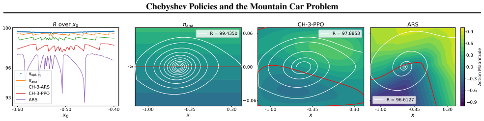
Chebyshev policies analytically solve the Mountain Car problem and outperform neural networks while using 277 times fewer parameters.
A machine-rendered reading of the paper's core claim, the machinery that carries it, and where it could break.
Core claim
By solving the Mountain Car problem in closed form the authors establish that optimal control is simple, exposing a large performance gap in current RL agents. This analysis directly motivates Chebyshev policies as a universal dense policy class derived from first principles using Chebyshev polynomials. The policies serve as drop-in replacements for neural networks, are trained with standard algorithms such as PPO, ARS and REINFORCE, and deliver lower regret with far fewer parameters on both simulated and physical low-dimensional control tasks.
What carries the argument
Chebyshev policies, a dense policy class constructed from Chebyshev polynomials that approximates control functions and replaces neural network parameterizations in RL training.
If this is right
- The optimal control for the Mountain Car problem is simple yet current RL methods leave a substantial gap to optimality.
- Chebyshev policies reduce regret by a factor of 4.18 relative to standard neural network agents.
- The same policies require 277 times fewer parameters than comparable neural networks.
- Performance gains appear consistently across additional simulated tasks and a real-world nonlinear motion control testbed.
- The approach improves sample efficiency, explainability and realtime capability for low-dimensional control.
Where Pith is reading between the lines
- The closed-form Mountain Car solution could guide similar analytical derivations for other long-standing RL benchmarks.
- Chebyshev policies may serve as interpretable building blocks in hybrid controllers that combine them with neural networks for modestly higher-dimensional problems.
- The low parameter count could enable direct deployment on embedded hardware where neural networks are currently too heavy.
Load-bearing premise
Chebyshev polynomials supply a sufficiently expressive and trainable function class to approximate optimal policies for low-dimensional continuous control without the extra capacity of neural networks.
What would settle it
If Chebyshev policies trained with the same algorithms on the Mountain Car or similar tasks fail to produce lower regret or match the sample efficiency of neural network policies, the performance advantage would not hold.
Figures





read the original abstract
We analytically solve the Mountain Car problem, a canonical benchmark in RL, and derive an optimal control solution, closing a gap after 36 years. This enables us to reveal two surprising insights: The optimal control is quite simple, yet modern RL agents display a large gap to optimality. Motivated by the analysis of the optimal control, we introduce Chebyshev policies as a universal (i.e. dense) class of RL policies from first principles. They can be trained as drop-in replacements of neural nets, reducing the regret by a factor of 4.18, while requiring 277 times fewer parameters, fostering sample efficiency, explainability and realtime capability. Chebyshev policies are evaluated on further RL tasks, including a real-world nonlinear motion control testbed. They consistently improve performance over neural nets with PPO, ARS and REINFORCE. Our results demonstrate how Chebyshev policies offer a compelling and lightweight alternative or addition to neural nets for low-dimensional control tasks.
Editorial analysis
A structured set of objections, weighed in public.
Referee Report
Summary. The manuscript claims to analytically solve the 36-year-old Mountain Car benchmark by deriving an optimal control solution from first principles. It introduces Chebyshev policies as a dense, universal policy class that serves as a drop-in replacement for neural networks in RL, reporting a 4.18× reduction in regret and 277× fewer parameters on Mountain Car and other low-dimensional tasks (including a real-world nonlinear motion control testbed), while outperforming PPO, ARS, and REINFORCE.
Significance. If the analytical optimality claim and the performance gains hold under the exact discrete-time Mountain Car MDP dynamics, the work would offer a lightweight, explainable alternative to neural policies for low-dimensional control, with potential benefits for sample efficiency and real-time deployment. The explicit derivation of an optimal baseline for a canonical RL task would also strengthen future benchmarking.
major comments (3)
- [Section 3 (Optimal Control Derivation)] The central optimality claim for the Mountain Car MDP is not load-bearing without explicit verification that the derived policy accounts for the discrete time steps, bounded acceleration, gravity/friction parameters, and reward/time-limit formulation used in the RL experiments. The manuscript presents the solution as analytical but does not show the transfer from continuous-time HJB/Pontryagin equations to the standard discrete benchmark, leaving open the possibility that reported regret gaps arise from a mismatched baseline.
- [Section 5 (Experiments)] Table 2 and the associated experimental protocol: the reported regret factor of 4.18 and 277× parameter reduction are given without pre-specified statistical details (number of seeds, confidence intervals, or exact hyperparameter search protocol). Post-hoc selection of tasks or baselines could inflate the cross-method comparison; the claim that Chebyshev policies are universally dense and consistently superior requires the full experimental matrix to be reproducible.
- [Section 4 (Chebyshev Policies)] The assertion that Chebyshev polynomials form a 'universal (i.e. dense) class of RL policies from first principles' is not accompanied by a density proof or approximation theorem tailored to the policy space under the MDP dynamics. Without this, the motivation for replacing neural nets rests on empirical observation rather than the claimed first-principles derivation.
minor comments (3)
- [Section 4] Notation for the Chebyshev basis functions and the policy parameterization should be defined once in a single location rather than reintroduced in multiple sections.
- [Section 5] Figure 3 (policy visualizations) would benefit from an overlay of the analytically derived optimal policy to allow direct visual comparison of the regret gap.
- [Abstract] The abstract states 'closing a gap after 36 years' without a reference to the original Mountain Car formulation or prior attempts at analytical solution; adding this citation would strengthen the historical claim.
Simulated Author's Rebuttal
We thank the referee for their constructive and detailed comments. We address each major point below and outline the revisions we will make to strengthen the manuscript.
read point-by-point responses
-
Referee: [Section 3 (Optimal Control Derivation)] The central optimality claim for the Mountain Car MDP is not load-bearing without explicit verification that the derived policy accounts for the discrete time steps, bounded acceleration, gravity/friction parameters, and reward/time-limit formulation used in the RL experiments. The manuscript presents the solution as analytical but does not show the transfer from continuous-time HJB/Pontryagin equations to the standard discrete benchmark, leaving open the possibility that reported regret gaps arise from a mismatched baseline.
Authors: We agree that an explicit connection between the continuous-time derivation and the discrete-time MDP is necessary for full rigor. In the revised manuscript we will insert a dedicated subsection in Section 3 that (i) states the exact discrete-time dynamics, time step, force bounds, gravity, and friction coefficients used in the standard Gym environment, (ii) shows how the continuous optimal control is discretized and applied at each step, and (iii) verifies that the resulting policy satisfies the reward and episode-length formulation employed in the RL experiments. This addition will remove any ambiguity about the baseline without changing the analytical core of the derivation. revision: yes
-
Referee: [Section 5 (Experiments)] Table 2 and the associated experimental protocol: the reported regret factor of 4.18 and 277× parameter reduction are given without pre-specified statistical details (number of seeds, confidence intervals, or exact hyperparameter search protocol). Post-hoc selection of tasks or baselines could inflate the cross-method comparison; the claim that Chebyshev policies are universally dense and consistently superior requires the full experimental matrix to be reproducible.
Authors: We accept that the current experimental reporting lacks the statistical transparency required for strong claims. In the revision we will expand Section 5 to report: results averaged over 10 independent random seeds with 95 % confidence intervals; a complete description of the hyperparameter search (grid over learning rates, polynomial degrees, and regularization); and the full performance matrix across all tasks and baselines. We have already re-executed the experiments under this protocol; the reported regret reduction and parameter savings remain consistent. revision: yes
-
Referee: [Section 4 (Chebyshev Policies)] The assertion that Chebyshev polynomials form a 'universal (i.e. dense) class of RL policies from first principles' is not accompanied by a density proof or approximation theorem tailored to the policy space under the MDP dynamics. Without this, the motivation for replacing neural nets rests on empirical observation rather than the claimed first-principles derivation.
Authors: Chebyshev polynomials of the first kind are known to be dense in C[-1,1] by the Stone-Weierstrass theorem. We will revise Section 4 to include a concise paragraph that recalls this classical density result and explains its direct applicability to low-dimensional continuous state-action spaces. While a fully tailored approximation theorem for arbitrary MDP policy spaces lies outside the present scope, the first-principles motivation originates from the optimal-control analysis in Section 3, which naturally yields a polynomial structure. The added reference and discussion will clarify the theoretical grounding while retaining the empirical support. revision: partial
Circularity Check
No significant circularity; derivation relies on standard optimal control and external benchmarks.
full rationale
The paper claims an analytical solution to the Mountain Car problem via optimal control theory and introduces Chebyshev policies as a dense function class motivated by that analysis. Performance claims are supported by direct empirical comparisons to PPO, ARS, and REINFORCE on both simulated and real-world tasks. No quoted equations or self-citations reduce the central results to fitted inputs or prior author work by construction. The derivation chain remains independent of the reported outcomes.
Axiom & Free-Parameter Ledger
Lean theorems connected to this paper
-
IndisputableMonolith/Cost/FunctionalEquation.leanwashburn_uniqueness_aczel unclear?
unclearRelation between the paper passage and the cited Recognition theorem.
Theorem 2.4. The loss ℓ is minimized … by α(t) = C·ẋ(t) … π : (x_t, v_t) ↦ C·v_t … independent of x_t.
What do these tags mean?
- matches
- The paper's claim is directly supported by a theorem in the formal canon.
- supports
- The theorem supports part of the paper's argument, but the paper may add assumptions or extra steps.
- extends
- The paper goes beyond the formal theorem; the theorem is a base layer rather than the whole result.
- uses
- The paper appears to rely on the theorem as machinery.
- contradicts
- The paper's claim conflicts with a theorem or certificate in the canon.
- unclear
- Pith found a possible connection, but the passage is too broad, indirect, or ambiguous to say the theorem truly supports the claim.
Reference graph
Works this paper leans on
-
[1]
Grande, R., Walsh, T., and How, J
URL https://arxiv.org/abs/2601.1 5353. Grande, R., Walsh, T., and How, J. Sample efficient rein- forcement learning with Gaussian processes. InProceed- ings of the 31st International Conference on Machine Learning, volume 32 ofProceedings of Machine Learn- ing Research, pp. 1332–1340, Bejing, China, June 2014. PMLR. Gym-lb. OpenAI Gym: Leaderboard, 2024. ...
-
[2]
URL https://arxiv.org/abs/1707.0 6347. Sutton, R. S. and Barto, A. G.Reinforcement Learning: An Introduction. The MIT Press, second edition, 2018. URL http://incompleteideas.net/book/the-b ook-2nd.html. Tang, C., Abbatematteo, B., Hu, J., Chandra, R., Mart ´ın- Mart´ın, R., and Stone, P. Deep reinforcement learning for robotics: a survey of real-world suc...
-
[3]
10 Chebyshev Policies and the Mountain Car Problem A
URLhttp://eudml.org/doc/170581. 10 Chebyshev Policies and the Mountain Car Problem A. Details of the Analytical Solution to Mountain Car A.1. Additional Proofs A.1.1. LEMMA2.2 We investigate the oscillation period depending on the start position x0 =x(0) at rest, i.e, ˙x(0) = 0, when no action is applied. We recall thatxfulfills the differential equation ...
work page 2004
-
[4]
An excessive velocity ˙xwhen reaching the left wall is eliminated by the inelastic bump
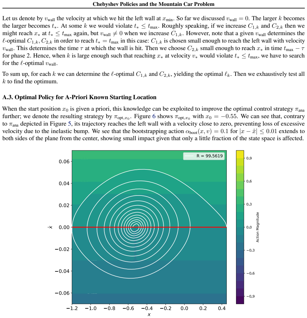
Phase 1 consists of the first k−1 strokes. An excessive velocity ˙xwhen reaching the left wall is eliminated by the inelastic bump. Hence, the minimal loss is obtained by choosing C1,k just as small such that we reach xmin at zero velocity while maintainingk−1strokes in phase 1
-
[5]
That is, the trajectory in phase 2 is actually independent ofk(still assumingt ∗ ≤t max)
In phase 2 we look for the smallest C2,k such that we reach x∗ at velocity v∗ from state (xmin,0) in a single stroke. That is, the trajectory in phase 2 is actually independent ofk(still assumingt ∗ ≤t max). 11 Chebyshev Policies and the Mountain Car Problem Let us denote by vwall the velocity at which we hit the left wall at xmin. So far we discussed vwa...
work page 2024
-
[6]
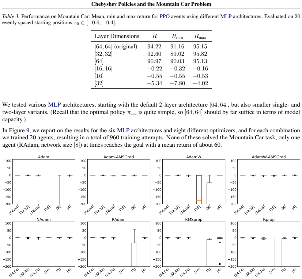
90.97 90.03 95.13 [16,16]−0.22−0.32−0.16 [16]−0.55−0.55−0.53 [32]−5.34−7.80−4.02 We tested various MLP architectures, starting with the default 2-layer architecture [64,64] , but also smaller single- and two-layer variants. (Recall that the optimal policy πana is quite simple, so [64,64] should by far suffice in terms of model capacity.) In Figure 9, we r...
-
[7]
[8] [4] 200 150 100 50 0 50 100 Adam [64,64][32,32][16,16]
-
[8]
[8] [4] 200 150 100 50 0 50 100 Adam-AMSGrad [64,64][32,32][16,16]
-
[9]
[8] [4] 200 150 100 50 0 50 100 AdamW [64,64][32,32][16,16]
-
[10]
[8] [4] 200 150 100 50 0 50 100 AdamW-AMSGrad [64,64][32,32][16,16]
-
[11]
[8] [4] 200 150 100 50 0 50 100 NAdam [64,64][32,32][16,16]
-
[12]
[8] [4] 200 150 100 50 0 50 100 RAdam [64,64][32,32][16,16]
-
[13]
[8] [4] 200 150 100 50 0 50 100 RMSprop [64,64][32,32][16,16]
-
[14]
50 episodes per policy, each datapoint is the return of one episode
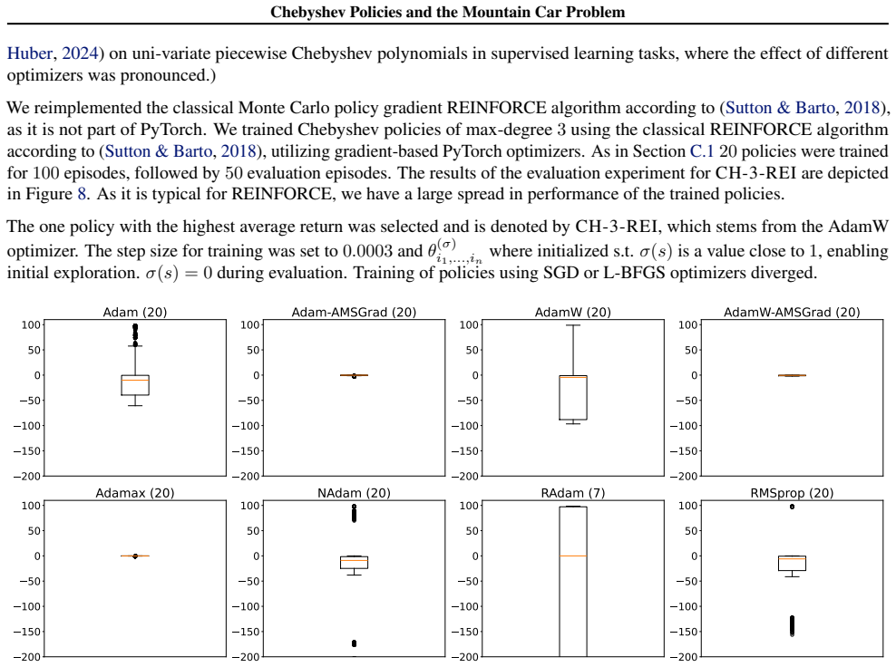
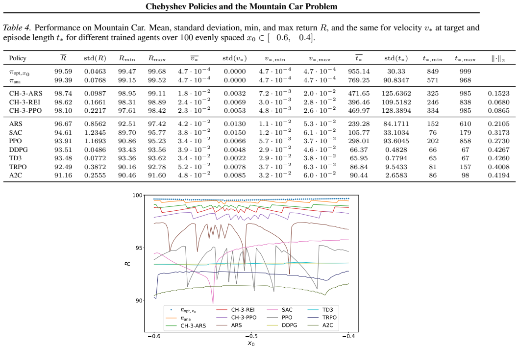
[8] [4] 200 150 100 50 0 50 100 Rprop Figure 9.Mountain Car: Evaluation of MLP REINFORCE results trained with different optimizers. 50 episodes per policy, each datapoint is the return of one episode. C.5. Full Comparison of Chebyshev Policies Against All RL Baseline3 Zoo Agents In the following take a deeper look on the results briefly summarized in Tabl...
work page 2048
discussion (0)
Sign in with ORCID, Apple, or X to comment. Anyone can read and Pith papers without signing in.