REVIEW 5 major objections 5 minor 1 cited by
A Multi-output Gaussian Process Regression with Negative Transfer Mitigation for Generating Boundary Test Scenarios of Multi-UAV Systems
T0 review · 5 major / 5 minor · reviewed 2026-08-07 · deepseek-v4-flash
Pith's one-line read Adaptive regularization of output-specific parameters steers multi-output Gaussian process training away from negative transfer and improves boundary test scenario generation for multi-UAV systems.
desk verdict A plausible new regularizer for LMC-based multi-output GPs, but the paper's headline claim of improvement on all outputs is contradicted by its own Table 4; deserves a serious referee but needs major revisions. read the letter →
The pith
A machine-rendered reading of the paper's core claim, the machinery that carries it, and where it could break.
The reading
What carries the argument
The load-bearing object is the adaptive regularization term on output-specific characteristic parameters. In LMC-based MOGPR, each output is a weighted sum of shared latent Gaussian processes, and the joint covariance is the Kronecker product $A \otimes K_x$ of a coregionalization matrix and an input kernel. The new term penalizes the squared L2 distance between paired per-output parameters, e.g., noise levels, with weights $w_k$ updated by Eq. (15): $w_k^{\mathrm{new}} \propto w_k \cdot \exp(-\lambda R(\boldsymbol{\theta}_{k1}, \boldsymbol{\theta}_{k2}))$ normalized over the parameter group, where $\lambda = 0.1$ and an early delay of 30 iterations prevents premature judgments. Every interval, the smallest active weight is frozen at $10^{-5}$, gradually releasing all constraints. This machinery converts a discrete question, which outputs are suffering negative transfer, into a continuous, automatically adjusted soft-sharing schedule that the optimizer can exploit.
What would settle it
Construct the two-output example from Section 3.1 and run MOGPR-NTM with the regularization weights frozen at a constant instead of updated by Eq. (15), sweeping lambda over a modest grid; if the fixed-weight version matches the adaptive version's RMSE, or if no lambda value reproduces the reported gains on the weak-signal output, then the adaptive mechanism is not doing the claimed work.
Extended reading notes
Core claim
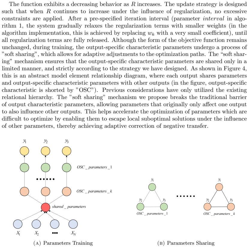
The central claim is that the failure mode behind negative transfer in LMC-based MOGPR is an optimization problem, not a modeling one: when outputs have imbalanced signal strengths and noise levels, the marginal likelihood has multiple local optima, and the optimizer can settle into one where the cross-covariance is misestimated and one output's strong signal contaminates the other. MOGPR-NTM modifies the objective to $\mathcal{L}_{\mathrm{total}} = \mathcal{L}_{\mathrm{MLL}} + \sum_k w_k \|\boldsymbol{\theta}_{k1} - \boldsymbol{\theta}_{k2}\|_2^2$, where each $\boldsymbol{\theta}$ is an output-specific characteristic parameter such as per-output noise, and $w_k$ is updated adaptively by a softmax-type rule over the relative inconsistency. The adaptive weights gently pull related parameter pairs together while leaving unrelated pairs effectively unpenalized, and the scheduled freezing of the smallest weights eventually releases all constraints. The authors claim that this soft sharing expands the search space of gradient optimization, lets difficult parameters escape suboptimal regions, and preserves the Kronecker-product efficiency of the LMC-based MOGPR.
Load-bearing premise
The load-bearing premise is that a penalty on pairwise differences between per-output parameters, with the paper's particular schedule of adaptive weights, reliably pulls the optimizer out of the local optimum that causes negative transfer; no proof or sensitivity analysis shows that this holds for parameter pairs beyond the motivating two-output example.
Editorial extensions
If this is right
- Training an LMC-based MOGPR with the added adaptive L2 penalty retains the separable Kronecker structure, so the computational savings of LMC are preserved while negative transfer is reduced.
- Boundary test scenario sampling guided by MOGPR-NTM should spread samples across disjoint high-gradient regions instead of over-concentrating them, because the surrogate no longer over-trusts one output's gradient estimate.
- The method treats all outputs equally, so it can be applied in settings where no prior knowledge identifies which metric is most important or which output is being corrupted.
- On the paper's numerical tests, MOGPR-NTM reduces test-set RMSE relative to conventional MOGPR by roughly 4 to 23 percent, about 7.2 percent on average, in the single-input cases and improves seven of nine outputs in the multi-input high-noise cases.
- Because the regularization is parameter-based rather than kernel-based, it can be combined with other kernel choices within the LMC family.
Reading between the lines
- A reader could test whether the adaptive schedule is essential by running the same L2 penalty with fixed weights; if fixed weights match the adaptive results, the updating rule in Eq. (15), not the penalty itself, is the real active ingredient.
- The mechanism suggests a natural extension to deep Gaussian processes and non-stationary kernels, where output-specific parameters also appear; the paper itself names this direction as future work.
- The strongest headline claim, simultaneous improvement for all outputs, is stronger than the tables show, so a fair test of the method would report paired comparisons across many random seeds and state how often each output improves, rather than only average RMSE.
Editorial analysis
A structured set of objections, weighed in public.
Referee Report
Summary. The paper proposes an adaptive regularization scheme for LMC-based multi-output Gaussian process regression (MOGPR) to mitigate negative transfer among outputs. The method penalizes pairwise l2 differences between output-specific characteristic parameters (e.g., noise levels) with weights adaptively updated via Eq. (15) and Algorithm 1, including a freeze schedule that relaxes the penalty during training. The authors validate the method on synthetic multi-output functions and a multi-UAV boundary test scenario generation case, reporting an average test RMSE reduction over conventional MOGPR of about 7.2%.
Significance. If the central claim were fully established, the method would be a useful, lightweight add-on to LMC-based MOGPR, improving predictive accuracy in settings with imbalanced output noise and offering a practical tool for adaptive sampling in boundary test scenario generation. Strengths include the use of held-out test sets, so the reported accuracy improvements are genuine predictions rather than fitted values; a concrete application to multi-UAV testing; and a method that retains LMC computational efficiency. However, the claimed 'simultaneous improvements across all outputs' is contradicted by the paper's own Table 4, and the lack of an ablation against fixed regularization and the lack of error bars leave the main contribution insufficiently supported.
major comments (5)
- [Abstract and Conclusion] The abstract and the Conclusion state that the method 'yields simultaneous improvements in predictive accuracy across all outputs' and 'maintains or even improves predictive accuracy for all outputs,' but Table 4 reports RMSE increases for two of nine outputs (G2O1: -7.96%, G3O1: -12.70%). The evidence supports improvement on most outputs and on average, not on all; the central claim should be downgraded or the abstract revised to match the reported results.
- [Method for Mitigating Negative Transfer / Case Verification] The claimed benefit of the adaptive weight schedule is not isolated: no experiment compares MOGPR-NTM against MOGPR with a fixed l2 penalty on the same parameter inconsistencies. Without this baseline, it is unknown whether the improvement arises from the adaptive mechanism or simply from any shrinkage of output-specific parameters. An ablation with a fixed penalty and matched hyperparameters is needed to support the paper's central contribution.
- [Case Verification] Tables 1-4 report single RMSE values with no error bars, standard deviations, or repeated random train/test splits; the sentence 'Three independent runs were performed' in Section 4 does not clarify whether each model was trained multiple times or whether different models are meant. Given the reported average improvement is about 7.2%, run-to-run variation could be of comparable size. Repeated-seed mean +/- standard deviation or confidence intervals, and ideally a paired test across outputs, should be reported.
- [Algorithm 1 and Eq. (15)] Eq. (15) defines the update as w_new = w * len(theta_k) * exp(-lambda R) / sum_{i!=j} exp(-lambda R) with the raw squared inconsistency R, while Algorithm 1 line 13 uses w_new = 3 * w * exp(-lambda r) / sum(exp(-lambda r)) with the normalized relative inconsistency r. These two rules are not equivalent, and the 'len(theta_k)' factor versus constant 3 and raw versus relative inconsistency change the training procedure. The exact method must be specified unambiguously for reproducibility.
- [Method for Mitigating Negative Transfer / Conclusion] Because Algorithm 1 eventually freezes every regularization weight to 1e-5, the final objective is effectively the standard LMC marginal likelihood; any claimed benefit must come from the optimization trajectory. The paper provides no diagnostic showing that this trajectory escapes negative-transfer local optima, and no sensitivity analysis for the hand-chosen hyperparameters (lambda=0.1, the 30-iteration delay, the freezing interval, the initial regularization weights, and the sampling weights g and v in Eq. (4)). This is load-bearing for the central claim that the method 'helps the model escape local optima'.
minor comments (5)
- [Case Verification (Table captions)] The caption of Table 1 reads 'Prediction of Single Input Loss under L2 Regularization' while Table 3 reads 'under L1 Regularization'; both are inconsistent with Eq. (14), which specifies an l2 penalty, and the second is likely a typo.
- [Title] The title contains a spacing error: 'A MUL TI-OUTPUT' should read 'A MULTI-OUTPUT'.
- [Method Motivation] The notation '2 epsilon_1 = epsilon_2 = 0.2' in Section 3.1 is unclear; please specify the noise standard deviations or scales for each output explicitly.
- [Algorithm 1 and text] The text mentions that regularization begins after 30 optimization iterations, but Algorithm 1's 'interval' parameter is never explicitly defined or set; specify its value in the experimental setup.
- [Figure 5] Figure 5, 'Iterations to Start Regularization,' is not cross-referenced in the text and its axes are unlabeled; please add a reference and axis labels.
Circularity Check
No circularity: held-out test-set RMSE comparisons are genuine predictions, adaptive weights are not fitted to test outputs, and the only self-citation is a non-load-bearing background review.
full rationale
The paper's derivation chain is not circular. MOGPR-NTM adds pairwise l2 penalties on output-specific characteristic parameters (e.g., output noise levels) to the marginal likelihood (Eq. 14), with weights adapted by Eq. (15)/Algorithm 1. All accuracy claims are evaluated as RMSE on held-out test subsets (Tables 1-4), so the predicted quantities are not constructed from the targets being predicted; the regularization hyperparameters (lambda=0.1, 30-iteration delay, freezing interval) are fixed choices rather than fitted to those test outputs. The abstract's 'simultaneous improvements across all outputs' is over-strong because Table 4 shows RMSE increases for G2O1 (-7.96%) and G3O1 (-12.70%), and the paper itself says 'Out of nine total predicted outputs ... seven outputs achieved optimized prediction performance'; this is an overclaim/correctness issue, not circularity. The paper also acknowledges that after the freezing schedule 'the form of the objective function remains unchanged' (all weights become 1e-5), so any claimed benefit must arise from the optimization trajectory rather than a modified final objective; this is an absence of theoretical guarantee/sensitivity analysis, not an equation-level reduction to inputs. Ref [1] includes author H. Yu but is cited only as general background on MUS T&E and carries none of the central argument, so it is not load-bearing. No fitted parameter is renamed as a prediction, no uniqueness theorem is imported from the authors' prior work, and no ansatz is smuggled in via citation. Therefore the circularity score is 0.
Assumptions & free parameters
free parameters (6)
- lambda (λ) =
0.1
- initial regularization weights w[key] =
unspecified positive values
- freezing interval =
unspecified ('interval')
- regularization delay =
30 iterations
- sampling weights g and v =
adjusted over iterations per Figure 9
- choice of regularized output-specific parameters =
e.g., output noise levels
assumptions (5)
- domain assumption LMC represents each output as a linear combination of independent latent GPs sharing an input kernel.
- ad hoc to paper Penalizing pairwise l2 inconsistency of output-specific parameters with adaptive weights mitigates negative transfer.
- ad hoc to paper The adaptive weight update in Eq. (15) improves optimization without biasing the final solution.
- domain assumption High-gradient regions of the surrogate output correspond to boundary test scenarios.
- domain assumption All MUS performance metrics are equally important.
Cite this review
Pith. "Pith review of A Multi-output Gaussian Process Regression with Negative Transfer Mitigation for Generating Boundary Test Scenarios of Multi-UAV Systems." pith.science (2026). https://pith.science/paper/4WER6I4P
@misc{pith2026250522331,
  author       = {Pith},
  title        = {Pith review of: A Multi-output Gaussian Process Regression with Negative Transfer Mitigation for Generating Boundary Test Scenarios of Multi-UAV Systems},
  year         = {2026},
  howpublished = {\url{https://pith.science/paper/4WER6I4P}},
  note         = {Machine review of arXiv:2505.22331}
}
read the original abstract
Adaptive sampling based on Gaussian process regression (GPR) has already been applied with considerable success to generate boundary test scenarios for multi-UAV systems (MUS). One of the key techniques in such researches is leveraging the accurate prediction of the MUS performance through GPR in different test scenarios. Due to the potential correlations among the multiple MUS performance metrics, current researches commonly utilize a multi-output GPR (MOGPR) to model the multiple performance metrics simultaneously. This approach can achieve a more accurate prediction, rather than modeling each metric individually. However, MOGPR still suffers from negative transfer. When the feature of one output variable is incorrectly learned by another, the models training process will be negatively affected, leading to a decline in prediction performance. To solve this problem, this paper proposes a novel adaptive regularization approach into the conventional MOGPR training process. Unlike existing regularization approaches for mitigating negative transfer in MOGPR, our method penalizes the inconsistencies among output-specific characteristic parameters using adaptively adjustable regularization weights. This mechanism helps each set of output parameters avoid local optima. Consequently, it yields simultaneous improvements in predictive accuracy across all outputs. Finally, we validate our approach on a numerical case and on a boundary test scenario generation case for a MUS multi-objectives search task.
Figures


Figures from the paper (15 more)


Forward citations
Cited by 1 Pith paper
-
AutoODD: Agentic Audits via Bayesian Red Teaming in Black-Box Models
AutoODD combines an LLM agent with per-axis Gaussian Process uncertainty to automatically discover failure modes of black-box models, demonstrated on missing-digit MNIST and aircraft detect-and-avoid.
Reference graph
Works this paper leans on
-
[1]
R. Zhao, H. Yu, Y. You, et al., Review on current status and technology method of unmanned swarm test evaluation, System Engineering and Electronics 46 (2) (2024) 570–
work page 2024
-
[2]
Z. Pan, C. Zhang, Y. Xia, H. Xiong, X. Shao, An improved artificial potential field method for path planning and formation control of the multi-uav systems, IEEE Transactions on Circuits and Systems II: Express Briefs 69 (3) (2022) 1129–1133. doi:10.1109/TCSII. 2021.3112787
arXiv 2022
-
[3]
M. Sarkar, X. Yan, S. Nateghi, B. J. Holmes, K. G. Vamvoudakis, A. Homaifar, A frame- work for testing and evaluation of operational performance of multi-uav systems, in: K. Arai (Ed.), Intelligent Systems and Applications, Springer International Publishing, Cham, 2022, pp. 355–374
work page 2022
-
[4]
J. Wubben, J. P. Matos-Carvalho, D. Pedro, S. Tomic, C. T. Calafate, Empirical eval- uation of multi uav coverage path planning for aerial surveying, in: 2024 20th Interna- tional Conference on Distributed Computing in Smart Systems and the Internet of Things (DCOSS-IoT), 2024, pp. 277–284. doi:10.1109/DCOSS-IoT61029.2024.00050
-
[5]
W. Sui, Q. Ma, H. Qiu, J. Hu, X. Yu, W. Chen, Research on mission capability testing and evaluation system of uav swarm, in: 2023 China Automation Congress (CAC), 2023, pp. 8926–8931. doi:10.1109/CAC59555.2023.10450439
arXiv 2023
-
[6]
P. Twu, R. Chipalkatty, J.-P. de la Croix, T. Ramachandran, J. Shively, M. Egerstedt, A. Rahmani, R. Young, A hardware testbed for multi-uav collaborative ground convoy protection in dynamic environments, in: AIAA modeling and simulation technologies con- ference, 2011. doi:10.2514/6.2011-6665
- [7]
-
[8]
F. Sahebsara, M. Snellgrove, M. De Queiroz, A low-cost experimental testbed for decen- tralized control of multi-uav systems, in: 2024 IEEE Conference on Control Technology and Applications (CCTA), 2024, pp. 351–356. doi:10.1109/CCTA60707.2024.10666654
arXiv 2024
Show all 49 references
-
[9]
Santana, R
E. Santana, R. Moreno, C. S´ anchez, M. A. Piera, A framework for multi-uav software in the loop simulations, International Journal of Service and Computing Oriented Manufacturing 3 (2-3) (2018) 190–211. doi:10.1504/IJSCOM.2018.091613
2018
-
[10]
S. Feng, H. Sun, X. Yan, H. Zhu, Z. Zou, S. Shen, H. X. Liu, Dense reinforcement learning for safety validation of autonomous vehicles, Nature 615 (7953) (2023) 620–627. doi: 10.1038/s41586-023-05732-2
2023 doi
-
[11]
Schmidt, A
T. Schmidt, A. Pretschner, Stellauav: A tool for testing the safe behavior of uavs with scenario-based testing (tools and artifact track), in: 2022 IEEE 33rd Interna- tional Symposium on Software Reliability Engineering (ISSRE), 2022, pp. 37–48. doi: 10.1109/ISSRE55969.2022.00015
2022
-
[12]
Daoud, C
A. Daoud, C. Bunel, M. Gu´ eriau, Cornersim: A virtualization framework to generate real- istic corner-case scenarios for autonomous driving perception testing, Procedia Computer Science 238 (2024) 184–191. doi:10.1016/j.procs.2024.06.014
2024 doi
-
[13]
B. Zhu, P. Zhang, J. Zhao, W. Deng, Hazardous scenario enhanced generation for au- tomated vehicle testing based on optimization searching method, IEEE Transactions on Intelligent Transportation Systems 23 (7) (2022) 7321–7331. doi:10.1109/TITS.2021. 3068784
2022 doi
-
[14]
G. E. Mullins, P. G. Stankiewicz, R. C. Hawthorne, S. K. Gupta, Adaptive generation of challenging scenarios for testing and evaluation of autonomous vehicles, Journal of Systems and Software 137 (2018) 197–215
2018
-
[15]
G. E. Mullins, P. G. Stankiewicz, M. A. Huntley, Search-based testing methods for eval- uating the resilience of autonomous unmanned underwater vehicles, Johns Hopkins APL Technical Digest (Applied Physics Laboratory) 34 (4) (2019) 497–510
2019
-
[16]
N.-C. Xiao, M. J. Zuo, W. Guo, Efficient reliability analysis based on adaptive sequential sampling design and cross-validation, Applied Mathematical Modelling 58 (2018) 404–420. doi:doi.org/10.1016/j.apm.2018.02.012
2018 doi
-
[17]
H. Liu, J. Cai, Y.-S. Ong, Remarks on multi-output gaussian process regression, Knowledge-Based Systems 144 (2018) 102–121
2018
-
[18]
E. V. Bonilla, K. Chai, C. Williams, Multi-task gaussian process prediction, Advances in neural information processing systems 20 (2007)
2007
-
[19]
Joukov, D
V. Joukov, D. Kuli´ c, Fast approximate multioutput gaussian processes, IEEE Intelligent Systems 37 (4) (2022) 56–69. doi:10.1109/MIS.2022.3169036
2022
-
[20]
Gardner, G
J. Gardner, G. Pleiss, K. Q. Weinberger, D. Bindel, A. G. Wilson, Gpytorch: Black- box matrix-matrix gaussian process inference with gpu acceleration, Advances in neural information processing systems 31 (2018)
2018
-
[21]
K. Das, A. N. Srivastava, Sparse inverse kernel gaussian process regression, Statistical Analysis and Data Mining: The ASA Data Science Journal 6 (3) (2013) 205–220. doi: 10.1002/sam.11189
2013 doi
-
[22]
Snelsoa, Sparse gaussian processes using pseudo-inputs, Advances in Neural Infor- mattmˆ Processing Systems 18 (2006) 1259–1266
E. Snelsoa, Sparse gaussian processes using pseudo-inputs, Advances in Neural Infor- mattmˆ Processing Systems 18 (2006) 1259–1266
2006
-
[23]
T. Ding, R. Zheng, S. Zhang, M. Liu, Resource-efficient cooperative online scalar field map- ping via distributed sparse gaussian process regression, IEEE Robotics and Automation Letters 9 (3) (2024) 2295–2302. doi:10.1109/LRA.2024.3355782
2024
-
[24]
L. Yang, K. Wang, L. Mihaylova, Online sparse multi-output gaussian process regression and learning, IEEE Transactions on Signal and Information Processing over Networks 5 (2) (2019) 258–272. doi:10.1109/TSIPN.2018.2885925
2019
-
[25]
Cheng, M
Z. Cheng, M. Li, G. Jia, Z. Shi, Adaptive gaussian process with pca for prediction of com- plex dispersion relations for periodic structures, European Journal of Mechanics - A/Solids 93 (2022) 104547. doi:https://doi.org/10.1016/j.euromechsol.2022.104547
2022
-
[26]
Z. Zhai, H. Li, X. Wang, An adaptive sampling method for kriging surrogate model with multiple outputs, Engineering with Computers 38 (2020) 277–295. doi:10.1007/ s00366-020-01145-1
2020
-
[27]
S. J. Pan, Q. Yang, A survey on transfer learning, IEEE Transactions on Knowledge and Data Engineering 22 (10) (2010) 1345–1359. doi:10.1109/TKDE.2009.191
2010 doi
-
[28]
G. Leen, J. Peltonen, S. Kaski, Focused multi-task learning using gaussian processes, in: Lecture Notes in Computer Science (including subseries Lecture Notes in Artificial Intelligence and Lecture Notes in Bioinformatics), Vol. 6912 (Part 2), 2011, pp. 310–325. doi:10.1007/97...
2011 doi
-
[29]
F. Chu, J. Wang, C. Peng, R. Jia, D. He, F. Wang, Multi-source domains transfer learning strategy based on similarity measurement for batch process quality prediction, Canadian Journal of Chemical Engineering 101 (4) (2023) 2018–2032. doi:10.1002/cjce.24657
2023 doi
-
[30]
Alvarez, N
M. Alvarez, N. D. Lawrence, Sparse convolved gaussian processes for multi-output re- gression, in: Proceedings of the 22nd International Conference on Neural Information Processing Systems (NIPS 2008), NIPS’08, Curran Associates Inc., Red Hook, NY, USA, 2008, pp. 57–64
2008
-
[31]
Feinberg, L.-F
V. Feinberg, L.-F. Cheng, K. Li, B. E. Engelhardt, Large linear multi-output gaussian process learning (2017). arXiv:1705.10813
2017 arXiv
-
[32]
Lawrence, A
N. Lawrence, A. Hyv¨ arinen, Probabilistic non-linear principal component analysis with gaussian process latent variable models, Journal of Machine Learning Research 6 (11) (2005) 1783–1816
2005
-
[33]
Kontar, G
R. Kontar, G. Raskutti, S. Zhou, Minimizing negative transfer of knowledge in multivariate gaussian processes: A scalable and regularized approach, IEEE transactions on pattern analysis and machine intelligence 43 (10) (2020) 3508–3522
2020
-
[34]
M. Li, R. Kontar, On negative transfer and structure of latent functions in multioutput gaussian processes, SIAM/ASA Journal on Uncertainty Quantification 10 (4) (2022) 1714– 1732
2022
-
[35]
M. A. ´Alvarez, N. D. Lawrence, Computationally efficient convolved multiple output gauss- ian processes, Journal of Machine Learning Research 12 (41) (2011) 1459–1500
2011
-
[36]
S. D. Oman, B. Vakulenko-Lagun, A remark on the use of a weight matrix in the linear model of coregionalization, Mathematical Geosciences 44 (6) (2012) 505–512. doi:10. 1007/s11004-011-9370-5
2012
-
[37]
M. A. Alvarez, L. Rosasco, N. D. Lawrence, et al., Kernels for vector-valued functions: A review, Foundations and Trends® in Machine Learning 4 (3) (2012) 195–266
2012
-
[38]
P. Wei, F. Liu, C. Tang, Reliability and reliability-based importance analysis of structural systems using multiple response gaussian process model, Reliability Engineering & System Safety 175 (2018) 183–195. doi:10.1016/j.ress.2018.03.013
2018 doi
-
[39]
C.-Y. Li, B. Rakitsch, C. Zimmer, Safe active learning for multi-output gaussian processes, in: G. Camps-Valls, F. J. R. Ruiz, I. Valera (Eds.), Proceedings of The 25th International Conference on Artificial Intelligence and Statistics, Vol. 151 of Proceedings of Machine Learn...
2022
-
[40]
Goovaerts, Geostatistics for natural resources evaluation, Oxford university press, 1997
P. Goovaerts, Geostatistics for natural resources evaluation, Oxford university press, 1997
1997
-
[41]
X. Lyu, D. Huang, L. Wu, D. Chen, An adaptive multi-output gaussian process surrogate model for large-scale parameter estimation problems, Engineering Computations 41 (6) (2024) 162. doi:10.1108/EC-10-2023-0719
2024 doi
-
[42]
G. Yu, N. Li, C. Chen, X. Zhang, A novel global prediction framework for multi-response models in reliability engineering using adaptive sampling and active subspace methods, Computer Methods in Applied Mechanics and Engineering 433 (2025) 117506. doi:10. 1016/j.cma.2024.117506
2025
-
[43]
TYAN, J.-W
M. TYAN, J.-W. LEE, Efficient multi-response adaptive sampling algorithm for construc- tion of variable-fidelity aerodynamic tables, Chinese Journal of Aeronautics 32 (3) (2019) 547–558. doi:10.1016/j.cja.2018.12.012
2019 doi
-
[44]
Kanagawa, P
M. Kanagawa, P. Hennig, D. Sejdinovic, B. K. Sriperumbudur, Gaussian processes and ker- nel methods: A review on connections and equivalences, arXiv preprint arXiv:1807.02582 (2018)
2018 arXiv
-
[45]
J. Lu, Q. J. Wang, N. Fraehr, X. Xiang, X. Wu, Choice of gaussian process kernels used in lsg models for flood inundation predictions, Journal of Hydrology (2025) 132949
2025
-
[46]
R. Yao, S. Du, T. Wan, W. Cui, Y. Yang, Y. Jing, C. Li, Robust registration algorithm based on rational quadratic kernel for point sets with outliers and noise, Multimedia Tools and Applications 80 (2021) 27925 – 27945. doi:10.1007/s11042-021-10851-x
2021 doi
-
[47]
Y. Li, Q. Zhou, Pairwise meta-modeling of multivariate output computer models using nonseparable covariance function, Technometrics 58 (4) (2016) 483–494. Changsha, China Email address: jianghanxu19@nudt.edu.cn
2016
-
[581]
doi:10.12305/j.issn.1001-506X.2024.02.21
2024 doi
-
[4004]
doi:10.1007/s00170-019-03791-2
Reviewed August 7, 2026 · model on record in the stance chip above.
Discussion (0). Sign in to comment.