REVIEW 2 major objections 5 minor 1 cited by
A More Precise Elbow Method for Optimum K-means Clustering
T0 review · 2 major / 5 minor · reviewed 2026-08-09 · deepseek-v4-flash
Pith's one-line read The paper claims that the elbow point in k-means can be identified exactly by minimizing the tangent of the upward-facing corner angle, computed from three consecutive SSE values.
desk verdict The rational-form elbow formula is a neat pedagogical simplification, but the method misses its stated goal because the angle criterion is scale-dependent and the validation is circular. read the letter →
The pith
A machine-rendered reading of the paper's core claim, the machinery that carries it, and where it could break.
The reading
What carries the argument
The carrying object is the tangent of the upward-facing corner angle, $\tan(\psi_k)$, defined for each interior point $k$ by the formula above. It comes from the angle-between-two-lines identity, and the derivative $\sec^2 \psi$ shows that $\tan \psi$ is strictly increasing on $(90^\circ, 180^\circ)$, so the minimizing tangent equals the angle closest to 90 degrees. The additional constraint $m_{l_k} > m_{l_{k-1}}$, where $m_{l_k} = SSE(k+1) - SSE(k)$, filters out corners that face downward in the sense of growing SSE drops, preventing the algorithm from selecting a point after which the SSE still falls sharply.
What would settle it
Run the formula on a synthetic dataset whose true cluster count is known, then repeat after multiplying every $SSE(k)$ by a constant; if the selected $k$ changes, the method depends on arbitrary vertical scaling, contradicting its motivation. A simpler check: if the argmin of $\tan(\psi_k)$ is not the number of true components in a well-separated mixture, the angle criterion itself fails.
Extended reading notes
Core claim
The central result is Theorem 2.5: with $SSE(k)$ monotonically decreasing, the elbow point is $(k, SSE(k))$ that minimizes $\tan(\psi_k)$ over $k = 2, \ldots, n-1$ satisfying $m_{l_k} > m_{l_{k-1}}$, where $$\tan(\psi_k) = \frac{-SSE(k+1) + 2SSE(k) - SSE(k-1)}{1 + (SSE(k)-SSE(k-1))(SSE(k+1)-SSE(k))}.$$ The angle $\psi_k$ is the upward-facing angle at the corner formed by connecting consecutive SSE points; it always lies between 90 and 180 degrees under the flattening assumption, and $\tan$ is increasing on that interval, so the smallest (most negative) tangent is the angle closest to 90 degrees. The slope condition $m_{l_k} > m_{l_{k-1}}$ excludes corners at which the drop from $k$ to $k+1$ is at least as large as the drop from $k-1$ to $k$, because those points are not the start of a flattening tail. The authors derive the formula from the analytic-geometry identity for the angle between two lines, using the difference of slopes divided by one plus the product of slopes.
Load-bearing premise
The load-bearing premise is that the upward-facing angle closest to 90 degrees—computed from raw SSE slopes with no normalization—marks the true elbow, a heuristic that is stated rather than derived from cluster quality or stability.
Editorial extensions
If this is right
- Choosing $k$ reduces to evaluating a rational expression in three consecutive SSE values, so any system that can compute SSE can implement the method.
- The method automatically rejects candidates where the SSE drop is still increasing, avoiding the false elbow that can appear when a plot is drawn with a distorted vertical scale.
- Because no trigonometric inverse or logarithm is involved, the algorithm ports to programming languages and embedded environments that lack math libraries.
- The same tangent array can be plotted as a diagnostic: the minimizing $k$ is the elbow, and the tangent values show how much each candidate misses the 90-degree ideal.
- If the formula is adopted, cluster-count selection for k-means becomes reproducible: two analysts running the same SSE sequence get the same $k$.
Reading between the lines
- One consequence the paper leaves implicit is that the tangent formula is not invariant under vertical rescaling of SSE, so a preprocessing normalization (for example, dividing every $SSE(k)$ by $SSE(1)$) would make the chosen $k$ independent of plotting scale; the paper motivates its method with scaling distortion but does not include such a step.
- A testable extension is to benchmark the formula on synthetic data with known cluster structure against the silhouette and gap statistics, which the paper does not do; its own example only demonstrates a single data set.
- The algorithm as written breaks ties by returning the first $k$ that attains the minimum tangent; in cases where two $k$ values give very close tangents, a stability check across random k-means initializations would be a practical addition.
Signed reviews
Editorial analysis
A structured set of objections, weighed in public.
Referee Report
Summary. The manuscript proposes an automated elbow method for k-means clustering. It models the sequence (k, SSE(k)) as a polyline, defines at each interior point the upward-facing angle between the two adjacent segments, and selects as the elbow the point minimizing tan(ψ_k) among points where the consecutive SSE drops are decreasing (Theorem 2.5). The authors claim this makes the elbow method objective while using only arithmetic operations. They provide pseudocode, a Python implementation, and a single eight-point 2D example, from which they conclude that the optimal number of clusters is 6.
Significance. If the proposed criterion were valid, it would offer a simple and objective rule for choosing the number of k-means clusters, and the use of only arithmetic operations is a practical advantage over inverse-trigonometric or logarithmic alternatives. The paper is transparent about its derivation, ships no fitted parameters, and includes reproducible code, which are strengths. However, the central claim is undermined by a scale-invariance failure: the selected k changes when every SSE value is multiplied by a constant, even though such a rescaling leaves the k-means cluster assignments unchanged. Since the paper explicitly motivates the method by the distortions caused by arbitrary axis scaling, this is a load-bearing defect. The empirical validation is also limited to one illustrative dataset with visual confirmation rather than external criteria.
major comments (2)
- [Theorem 2.5, Eq. (4)] The proposed elbow criterion is not invariant under uniform rescaling of the SSE values, and this directly contradicts the paper's motivating problem of distorted axis scaling. Under the scaling SSE(k) -> c*SSE(k), every slope m_k becomes c*m_k, so tan(ψ_k) in Eq. (4) becomes c*(m_{k-1} - m_k)/(1 + c^2*m_{k-1}*m_k). Because the denominator changes nonlinearly, the ordering of the tangents can change. For example, take SSE = (100, 60, 40, 30, 28). For c = 1 the admissible tangents are approximately -0.025, -0.050, and -0.381 at k = 2, 3, 4, so the method selects k = 4. For c = 0.01, which corresponds to multiplying every SSE by 0.01 and hence to rescaling all data coordinates by 0.1, the tangents become approximately -0.185, -0.098, and -0.080, so the method selects k = 2. The condition m_k > m_{k-1} is satisfied in both cases. Uniform scaling of all coordinates leaves k-means assignments unchanged and multiplies SSE by c^2, so the same clustering problem yields different 'optimum' k. The manuscript provides no canonical normalization before applying Eq. (4), so the claimed objectivity fails.
- [Sections 2.1 and 2.3] The optimality premise that the elbow is the corner whose upward-facing angle is closest to 90 degrees is assumed rather than derived. Theorem 2.5 proves only a formula for that geometric quantity under the additional flattening condition; it does not connect the criterion to cluster quality, stability, separation, or any external notion of optimal k. The simulation in Section 2.3 uses the algorithm's own smallest tangent at k = 6 as evidence that k = 6 is correct, and the text then asserts that the k = 6 clustering in Figure 14 is better than the k = 3 clustering in Figure 15. There is no comparison with silhouette analysis, gap statistics, ground-truth labels, or any quantitative validation. Consequently, the manuscript's claim that the method gives 'a more reliable cluster determination' is not empirically supported.
minor comments (5)
- [Proposition 2.4] The final equivalence in the proof contains a sign error: the displayed expression should read SSE(k) - SSE(k + 1) >= SSE(k - 1) - SSE(k), not SSE(k) - SSE(k + 1) >= -SSE(k - 1) - SSE(k). The surrounding text uses the correct inequality.
- [Algorithm 1] The pseudocode for the SSE(k) function is incorrect as written: it loops only i = 1 to k over centroids and sums d(Xi, Ci), but it should sum over all n data points, assigning each point to its nearest centroid. The Python implementation uses kmeans.inertia_, so the code is correct, but the pseudocode does not match it.
- [Algorithm 2] The f-string print statement 'Tanpsi(i+1) = tanpsi[i]' will not produce the intended values when copied literally, and the variable name 'optimal k' should be 'optimal_k' for valid Python. These are presentation issues in an otherwise useful code listing.
- [Figures and text] Figure 15 has the placeholder caption 'Figure example', and there are several typographical errors throughout, including 'clusering', 'one oh such programming languages', 'Is is answered', and 'choses'. These should be corrected before publication.
- [Theorem 2.5 assumptions] The theorem assumes SSE(k+1) <= SSE(k), but k-means can produce equal SSE values across neighboring k; the algorithm sets tanpsi[k] = 0 in such cases, and the first such index is then returned as the optimum, which is an arbitrary tie-breaking rule. The claim that the algorithm 'considers every possibility of the elbow method graph behaviour' is therefore not fully justified.
Circularity Check
Partial circularity: the 'optimum k' is the closest-to-90° heuristic restated, and the validation reduces to the same monotone SSE input used to select k.
-
self definitional
[Section 2.1, Theorem 2.2 and Theorem 2.5]
"The elbow point is the point in which there is no significant drop of SSE afterwards. The typical elbow method determines the angle closest to 90◦ since it indicates the last point with a significant drop of SSE i.e. the graph starts flattening beyond the point. ... The elbow point is (k, SSE(k)) such that it satisfies min (tanψk|k = 2, 3, ..., n− 1)."
Theorem 2.2 and its refinement Theorem 2.5 present the elbow point as a mathematical conclusion, but the criterion 'closest to 90 degrees' is assumed as the meaning of elbow at the start of Section 2.1. The proof only shows that minimizing tan(ψk) selects the corner closest to 90 degrees on a monotone SSE curve; it never derives from cluster quality, stability, or information criteria that this corner is the optimum number of clusters. The theorem is therefore the heuristic premise restated in tangent form, so the claimed objective determination of optimum k is self-definitional rather than an independent derivation.
-
fitted input called prediction
[Section 2.3, discussion of Figures 14–15]
"In comparison to Figure 14, Figure 15 shows the k-means clustering if there are 3 clusters, mistakenly chosen by the biased Figure 11. We see that the clustering still leaves a huge distance between data points and their corresponding centroids. Figure 14 shows a better clustering where the distances are minimum."
The validation of k = 6 against k = 3 uses within-cluster distances as the measure of 'better clustering', but these distances are exactly the SSE values from which the elbow candidates were computed. The paper itself proves that SSE is monotonically decreasing as k increases, so any larger k trivially yields smaller distances. The comparison is therefore not independent evidence that 6 is optimal; it is a forced consequence of the same monotonicity assumption used to build the method. The predicted optimum is evaluated with the very input quantity that generated the prediction.
full rationale
The paper contains no fitted parameters, no self-citation chain, and the tangent formula in Eq. (4) is a correct analytic-geometry restatement. However, the central claim that the elbow point is the 'optimum' number of clusters is loaded into the formalism: the closest-to-90-degree corner is asserted as the definition of elbow, and Theorem 2.5 merely computes that corner. The subsequent demonstration that k = 6 gives smaller within-cluster distances than k = 3 is circular because the paper uses SSE both as the selection input and as the validation metric, while also asserting SSE decreases monotonically with k. The scale-dependence counterexample (multiplying SSE by a constant changes the argmin of tanψk) is a serious correctness flaw, but it is a matter of mathematical validity rather than circularity and is not counted in the score beyond the overall concern.
Assumptions & free parameters
assumptions (5)
- domain assumption SSE(k) is a strictly monotonically decreasing sequence over k = 1..n.
- ad hoc to paper The optimal number of clusters is the corner whose upward-facing angle is closest to 90 degrees, subject to decreasing drops.
- domain assumption The elbow graph is a piecewise-linear polyline connecting adjacent (k, SSE(k)) points with equal x-spacing 1.
- ad hoc to paper The condition m_k > m_{k-1} correctly identifies corners that may be elbows, and all other corners should be ignored.
- standard math tan(psi) is monotonically increasing on (90 degrees, 180 degrees), so the minimum tangent selects the angle closest to 90 degrees.
Cite this review
Pith. "Pith review of A More Precise Elbow Method for Optimum K-means Clustering." pith.science (2026). https://pith.science/paper/4YFA33DU
@misc{pith2026250200851,
  author       = {Pith},
  title        = {Pith review of: A More Precise Elbow Method for Optimum K-means Clustering},
  year         = {2026},
  howpublished = {\url{https://pith.science/paper/4YFA33DU}},
  note         = {Machine review of arXiv:2502.00851}
}
read the original abstract
K-means clustering is an unsupervised clustering method that requires an initial decision of number of clusters. One method to determine the number of clusters is the elbow method, a heuristic method that relies on visual representation. The method uses the number based on the elbow point, the point closest to 90 degrees that indicates the most optimum number of clusters. This research improves the elbow method such that it becomes an objective method. We use the analytical geometric formula to calculate an angle between lines and real analysis principle of derivative to simplify the elbow point determination. We also consider every possibility of the elbow method graph behaviour such that the algorithm is universally applicable. The result is that the elbow point can be measured precisely with a simple algorithm that does not involve complex functions or calculations. This improved method gives an alternative of more reliable cluster determination method that contributes to more optimum k-means clustering.
Figures


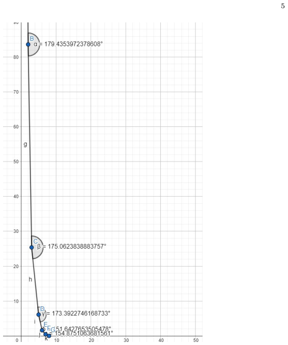
Figures from the paper (12 more)


Forward citations
Cited by 1 Pith paper
-
Beyond Random Partitioning: Unsupervised Spatio-Temporal Stratification for Cohort Balancing in Longitudinal Medical Imaging
K-means clustering on six intensity and temporal features plus intra-cluster stratified sampling reduces cross-subset imaging and temporal imbalance versus random splitting in a 149-patient longitudinal brain MRI cohort.
Reference graph
Works this paper leans on
-
[1]
Amelia, Indah Manfaati Nur, Muhammad Rizky, and Septiana Putri Milasari. Poverty level grouping in west java province with the k-means clustering method.Journal Of Data Insights, 1:51–61, 12 2023
work page 2023
- [2]
- [3]
-
[4]
Zeynep Karaca. The cluster analysis in the manufacturing industry with k-means method: An application for turkey.Eurasian Journal of Economics and Finance , 6:1–12, 9 2018
work page 2018
-
[5]
The parallel implementation and application of an improved k-means algorithm
X Li, L Yu, L Hang, and X Tang. The parallel implementation and application of an improved k-means algorithm. J. Univ. Electron. Sci. Technol , 46:61–68, 2017
work page 2017
-
[6]
Clustering algorithms in healthcare, 2021
Neerja Negi and Geetika Chawla. Clustering algorithms in healthcare, 2021
work page 2021
-
[7]
Data as oil, infrastructure or asset? three metaphors of data as economic value
Jan Michael Nolin. Data as oil, infrastructure or asset? three metaphors of data as economic value. Journal of Information, Communication and Ethics in Society , 18:28–43, 11 2019
work page 2019
-
[8]
Data clustering: application and trends
Gbeminiyi John Oyewole and George Alex Thopil. Data clustering: application and trends. Artificial Intelligence Review , 56:6439–6475, 7 2023
work page 2023
Show all 16 references
-
[9]
Springer International Publishing, 2017
Joe Pitt-Francis and Jonathan Whiteley.Guide to Scientific Computing in C++ . Springer International Publishing, 2017
2017
-
[10]
Sistem informasi data penduduk pada desa bogoharjo keca- matan ngadirojo kabupaten pacitan
Dwi Priyanti and Siska Iriani. Sistem informasi data penduduk pada desa bogoharjo keca- matan ngadirojo kabupaten pacitan. Indonesian Journal of Network & Security , 2:55–61, 2013
2013
-
[11]
Penerapan metode algoritma k-means clustering untuk pemetaan penyebaran penyakit demam berdarah dengue (dbd).JOURNAL OF SCIENCE AND SOCIAL RESEARCH , 4:336, 10 2021
Muhammad Ardiansyah Sembiring. Penerapan metode algoritma k-means clustering untuk pemetaan penyebaran penyakit demam berdarah dengue (dbd).JOURNAL OF SCIENCE AND SOCIAL RESEARCH , 4:336, 10 2021
2021
-
[12]
A quantitative discriminant method of elbow point for the optimal number of clusters in clustering algorithm
Congming Shi, Bingtao Wei, Shoulin Wei, Wen Wang, Hai Liu, and Jialei Liu. A quantitative discriminant method of elbow point for the optimal number of clusters in clustering algorithm. EURASIP Journal on Wireless Communications and Networking , 2021:31, 12 2021
2021
-
[13]
Sinaga and Miin-Shen Yang
Kristina P. Sinaga and Miin-Shen Yang. Unsupervised k-means clustering algorithm.IEEE Access, 8:80716–80727, 2020. 22
2020
-
[14]
Farming in kediri indonesia: analysis of cluster k-means
N Solikin, B Hartono, Sugiono, and Linawati. Farming in kediri indonesia: analysis of cluster k-means. IOP Conference Series: Earth and Environmental Science , 1041:012015, 6 2022
2022
-
[15]
Nanthyan Khampa Usada and Artha Prabawa. Analisis manajemen pengelolaan data sistem informasi puskesmas di tingkat dinas kesehatan di kabupaten bondowoso.Jurnal Biostatistik, Kependudukan, dan Informatika Kesehatan , 2:16, 11 2021
2021
-
[16]
Research on k-value selection method of k-means clustering algorithm
Chunhui Yuan and Haitao Yang. Research on k-value selection method of k-means clustering algorithm. J, 2:226–235, 6 2019
2019
Reviewed August 9, 2026 · model on record in the stance chip above.
Discussion (0). Continue with ORCID to comment.