REVIEW 3 major objections 4 minor 54 references
Hybridization fluctuations in the half-filled periodic Anderson model
T0 review · 3 major / 4 minor · reviewed 2026-08-14 · deepseek-v4-flash
Pith's one-line read The half-filled periodic Anderson model passes through an intermediate phase of hybridization fluctuations before the Kondo insulating state is established.
desk verdict A new observable and a plausible but not-yet-nailed-down intermediate phase; the paper earns a referee, not a desk reject. read the letter →
The pith
A machine-rendered reading of the paper's core claim, the machinery that carries it, and where it could break.
The reading
What carries the argument
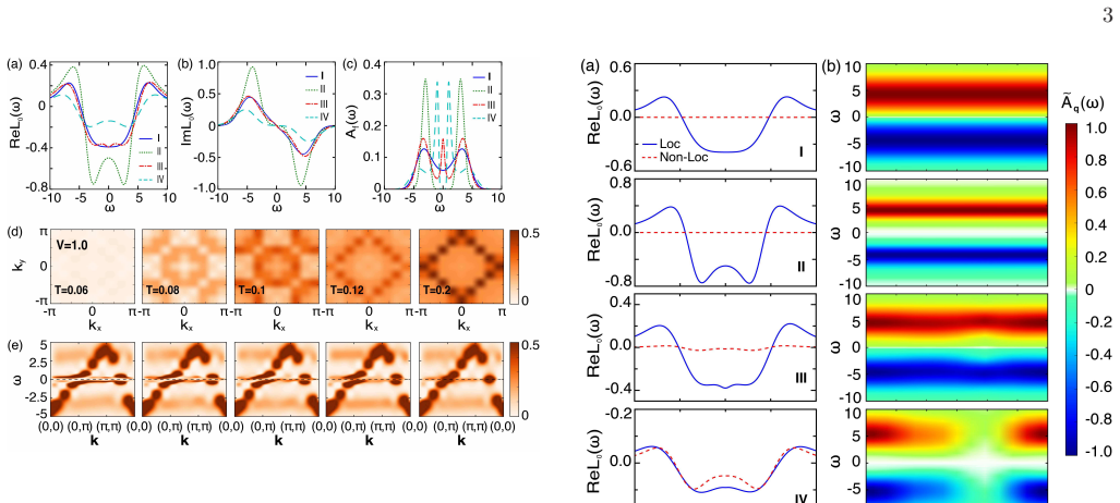
The central object is the dynamical hybridization correlation function $L_{ij}(\tau) = -\langle T_\tau[O_i(\tau)-\langle O_i\rangle][O_j(0)-\langle O_j\rangle]\rangle$, built from the local hybridization field $O_i=\sum_\sigma(c^\dagger_{i\sigma}f_{i\sigma}+f^\dagger_{i\sigma}c_{i\sigma})$ with the static average subtracted so that only fluctuations are followed. DQMC computes $L_q(\tau)$; the maximum entropy method continues it to the spectral function $A_q(\omega)=-\frac{1}{\pi}\mathrm{Im}\,L_q(\omega)$; Kramers-Kronig gives $\mathrm{Re}\,L_0(\omega)$. The load-bearing diagnostics are the shape of $\mathrm{Re}\,L_0(\omega)$ (one valley, two Hubbard valleys at $\pm U/2$, or a dip on a hump) and the low-energy slope $K=d\,\mathrm{Im}\,L_0(\omega)/d\omega|_{\omega=0}$, together with the decomposition of $\mathrm{Re}\,L_0(\omega)$ into local and nonlocal contributions. This machinery separates the thermal background of decoupled f and conduction electrons from genuine quantum hybridization fluctuations and traces how the latter grow into inter-site coherence.
What would settle it
Recompute the hybridization correlation function on a larger lattice (12×12 or 16×16) with more imaginary-time slices and continue it with a second method such as stochastic analytic continuation; if the dip in $\mathrm{Re}\,L_0(\omega)$ and the kink in $\mathrm{Im}\,L_0(\omega)$ in regime III do not persist, or if a direct large-$\tau$ fit of $L_0(\tau)$ shows a single exponential gap rather than a slow decay, the intermediate phase is an artifact of the maximum-entropy continuation.
Extended reading notes
Core claim
The central discovery is a four-regime crossover structure in the hybridization fluctuation spectrum $L_0(\omega)$ of the half-filled periodic Anderson model, obtained from DQMC on an $8\times8$ lattice. Regimes I and II are the decoupled thermal and selective-Mott limits, where $\mathrm{Re}\,L_0(\omega)$ shows one valley or two valleys at $\pm U/2$ and the low-energy slope of $\mathrm{Im}\,L_0(\omega)$ is small. Regime III is distinguished by a small dip in $\mathrm{Re}\,L_0(\omega)$, a large low-energy slope $K$ followed by a kink in $\mathrm{Im}\,L_0(\omega)$, and the onset of nonlocal (inter-site) hybridization correlations; the fermionic dispersion shows band bending but only a partially opened gap. Regime IV is the Kondo insulating state, where the direct hybridization gap is fully opened, the low-energy slope is suppressed, and the nonlocal contribution to $\mathrm{Re}\,L_0(\omega)$ becomes comparable to the local one. The paper concludes that lattice coherence is established only when sufficiently strong inter-site hybridization correlations develop at lower temperature, confirming the two-stage hybridization scenario proposed from experiments.
Load-bearing premise
The load-bearing assumption is that the small low-energy dip and kink in the maximum-entropy-continued hybridization spectrum on an $8\times8$ lattice are real physical features rather than artifacts of analytic continuation; if they are artifacts, the intermediate regime and the two-stage scenario lose their numerical foundation.
Editorial extensions
If this is right
- The Kondo insulating state of the half-filled periodic Anderson model should be viewed as a short-range-correlated insulator, not a simple mean-field band insulator; the nearest-neighbor hybridization correlation is its dominant nonlocal component.
- Band bending and a direct hybridization gap can appear while the system is still ungapped at the Fermi level, which explains ARPES and optical-conductivity signatures above the coherence temperature.
- The low-energy slope $K = d\,\mathrm{Im}\,L_0(\omega)/d\omega|_{\omega=0}$ is a nonmonotonic function of temperature for fixed $V$, so it can serve as a numerical diagnostic for locating the crossover boundaries between the four regimes.
- The two-stage hybridization scenario—fluctuation-dominated precursor followed by coherent Kondo insulator—is a generic feature of the half-filled periodic Anderson model in two dimensions, not a mean-field artifact.
- Hybridization fluctuations peak around $(\pi,\pi)$ in the Brillouin zone, indicating an interplay with magnetic fluctuations that may shape the coherence crossover.
Reading between the lines
- If the finite low-energy slope in regime III reflects a finite lifetime $\Gamma_k$ of the hybridization propagator, then the intermediate phase should exhibit a direct gap in optical conductivity while the indirect gap remains closed; measuring the temperature where the indirect gap opens would separate fluctuation-driven from coherence-driven physics.
- The near-$(\pi,\pi)$ weight of the normalized hybridization spectrum suggests checkerboard magnetic correlations assist hybridization; a testable extension is to compute the same $L_0(\omega)$ with frustration or next-nearest-neighbor hopping and see whether the intermediate regime widens or narrows.
- Because the phase diagram is read from the shape of $\mathrm{Re}\,L_0(\omega)$, the same diagnostic could be applied to cluster dynamical mean-field or tensor-network solutions of the Kondo lattice, giving a common language for comparing approximate methods.
- The nonmonotonic $K(T)$ could serve as a proxy for the hybridization coherence scale; comparing it with the temperature where the f-electron spectral weight at the Fermi level vanishes would quantify how much precursor fluctuation precedes full coherence.
Signed reviews
Editorial analysis
A structured set of objections, weighed in public.
Referee Report
Summary. This manuscript reports determinant Quantum Monte Carlo (DQMC) simulations of the half-filled periodic Anderson model on an 8x8 square lattice with U=6, t=1, and Ef=0. The authors define the local hybridization operator O_i and its imaginary-time correlation function L_ij(τ), then use the maximum entropy method to continue L_q(τ) to the hybridization spectral function, from which they obtain Re L_0(ω) via Kramers-Kronig. Based on the shape of Re L_0(ω) and Im L_0(ω), they identify four parameter regimes: a thermally dominated regime (I), a selective-Mott-like regime (II), an intermediate regime with low-energy hybridization fluctuations and band bending (III), and a Kondo insulating regime (IV). They further show that nonlocal hybridization correlations are negligible in regimes I-II, become visible in regime III, and grow to be comparable with local correlations in regime IV, predominantly near momentum (π,π). The paper concludes that the Kondo insulator forms only at lower temperatures through inter-site hybridization correlations and interprets this as numerical support for the two-stage hybridization scenario proposed by recent ARPES and pump-probe experiments.
Significance. The paper addresses a timely and important question: whether hybridization fluctuations produce a precursor regime above the Kondo insulating state, as suggested by recent ARPES and pump-probe experiments. Its main strength is that it computes the hybridization correlation function directly with sign-problem-free DQMC at half filling, without fitting parameters, and it provides useful analytic benchmarks in the V=0 limit (Eq. 4) and the mean-field limit (Eq. 5). If the regime III signature is physical, the work would be a valuable numerical step connecting hybridization fluctuations to photoemission, optical, and pump-probe observations. However, the central numerical evidence is not yet secured: the regime boundaries and the growth of nonlocal correlations are read from MaxEnt-continued spectra without error bars or continuation validation, so the significance is contingent on additional supportive tests.
major comments (3)
- [§2 and Figs. 1–4] The identification of regime III, the central claim of the paper, rests on small features in the MaxEnt-continued L0(ω): the dip in Re L0(ω) near ω=0, the kink in Im L0(ω) near |ω|≈0.2, and the slope K=d Im L0/dω at ω=0. The manuscript reports no statistical error bars on L0(ω) or K, no MaxEnt default-model or noise-level sensitivity tests, and no goodness-of-fit diagnostics for Eq. (3). Because MaxEnt can bias low-energy spectral weight depending on the default model and noise estimate, it is currently an open possibility that the dip/kink/slope features defining regime III are continuation artifacts rather than physical hybridization fluctuations. Please provide error bars and systematic MaxEnt validation (varying the default model, the noise estimate, and the number of time slices) for representative parameter sets in each regime.
- [Fig. 4] The phase boundaries in Fig. 4 are extracted 'roughly from the features of Re L0(ω)' with lines drawn as a guide to the eye, and the background color uses the slope K without any uncertainty. The right panel's nonmonotonic K(T) for V=1.0 is the only quantitative discriminator among the four regimes; without error bars or a stated criterion (e.g., zero crossing, dip depth threshold, slope threshold), the separation between regime III and regime IV is not quantitatively established. Please define the boundary criterion explicitly and provide uncertainties on K.
- [§2, finite-size statement] The only finite-size statement is that simulations 'were performed on an 8×8 square lattice with M=80 and examined with larger lattice size and time slices.' Because regime III is identified from low-energy features whose amplitude may be comparable to finite-size effects, and because the nonlocal correlation growth is dominated by nearest-neighbor terms, please show quantitative finite-size checks (e.g., K and the low-energy part of L0(ω) on 12×12 or 16×16 lattices) or explicitly quantify the systematic uncertainty from the lattice size.
minor comments (4)
- [Introduction] The phrase 'fluent-dependent relaxation' appears to be a typo for 'frequency-dependent relaxation'.
- [Fig. 2(d) and 2(e)] The intensity plots in Fig. 2(d) and 2(e) lack a color scale. Please specify the plotted quantity (e.g., spectral weight at the Fermi energy, A(k,ω=0)) and add a colorbar.
- [References] References 22 and 54 are arXiv preprints; please update them to published versions if available at the time of submission.
- [Abstract and text] The word 'consequentially' in the abstract is awkward; 'consequently' or 'as a result' would read more naturally. Similar phrasing appears in the main text.
Circularity Check
No substantive circularity: the DQMC spectra are first-principles computations with no fitted parameters; the only minor concern is interpretive self-citation to the authors' pump-probe preprint.
full rationale
The paper's central derivation is self-contained. It solves the half-filled periodic Anderson model by determinant Quantum Monte Carlo (Eqs. 1-3), computes the hybridization correlation function L_ij(tau), and analytically continues L_q(tau) to L_q(omega) with MaxEnt. No experimental data are fitted and no parameter is tuned to reproduce the claimed phase diagram; the regime boundaries are read off shape changes in Re L0(omega) and the slope K = d Im L0(omega)/domega at omega=0. Equations (4) and (5) are used only as analytic limiting forms to interpret the V=0 and mean-field Kondo-insulator spectra, not as inputs that force the classification. The identification of regime IV as a Kondo insulator is additionally corroborated by the gapped f-electron local DOS and momentum-resolved spectral function, so it is not defined by Eq. (5) alone. The conclusion 'confirms the two-stage hybridization scenario' cites the authors' own pump-probe preprint (Ref. 22), and Ref. 22 is used to frame the motivation; however, this self-citation is not load-bearing for the numerical derivation, since the DQMC spectra and MaxEnt continuation do not take the two-stage scenario as an input. The main weakness is numerical rather than circular: the low-energy dip and kink in regime III depend on MaxEnt continuation of 8x8 DQMC data without error bars or systematic default-model tests, so a MaxEnt artifact could alter the regime-III interpretation. That is a robustness concern, not a circularity of the derivation. No equation is defined in terms of the result it is said to predict, and no fitted quantity is renamed as a prediction.
Assumptions & free parameters
assumptions (4)
- standard math Determinant Quantum Monte Carlo with Hubbard-Stratonovich decoupling provides essentially exact imaginary-time correlation functions for the periodic Anderson model.
- domain assumption Maximum entropy analytic continuation reliably reproduces the low-energy features of Aq(omega).
- domain assumption An 8x8 lattice with M=80 time slices is representative of the thermodynamic limit at the temperatures studied.
- domain assumption The 2D half-filled periodic Anderson model captures the qualitative physics of heavy fermion materials probed by ARPES and pump-probe experiments.
Cite this review
Pith. "Pith review of Hybridization fluctuations in the half-filled periodic Anderson model." pith.science (2026). https://pith.science/paper/5MSSLYKY
@misc{pith2026190901846,
  author       = {Pith},
  title        = {Pith review of: Hybridization fluctuations in the half-filled periodic Anderson model},
  year         = {2026},
  howpublished = {\url{https://pith.science/paper/5MSSLYKY}},
  note         = {Machine review of arXiv:1909.01846}
}
read the original abstract
Motivated by recent photoemission and pump-probe experiments, we report determinant Quantum Monte Carlo simulations of hybridization fluctuations in the half-filled periodic Anderson model. A tentative phase diagram is constructed based solely on hybridization fluctuation spectra and reveals a crossover regime between an unhybridized selective Mott state and a fully hybridized Kondo insulating state. This intermediate phase exhibits nonlocal hybridization fluctuations and consequentially the so-called "band bending" and a direct hybridization gap as observed in angle-resolved photoemission spectroscopy and optical conductivity. This connects the band bending with the nonlocal hybridization fluctuations as proposed in latest ultrafast optical pump-probe experiment. The Kondo insulating state is only established at lower temperatures with the development of sufficiently strong inter-site hybridization correlations. Our work suggests a unified picture for interpreting recent photoemission, pump-probe, and optical observations and provides numerical evidences for the importance of hybridization fluctuations in heavy fermion physics.
Figures


Reference graph
Works this paper leans on
-
[1]
G. R. Stewart, Rev. Mod. Phys. 56, 755 (1984)
1984
-
[2]
A. C. Hewson, The Kondo Problem to Heavy Fermions, (Cambridge University Press, Cambridge, England, 1997)
work page 1997
-
[3]
Coleman, Introduction to Many-body Physics, (Cambridge University Press, Cambridge, England, 2015)
P. Coleman, Introduction to Many-body Physics, (Cambridge University Press, Cambridge, England, 2015)
work page 2015
-
[4]
Y. \= O nuki, Physics of Heavy Fermions: Heavy Fermions and Strongly Correlated Electrons Systems, (World Scientific Publishing, Singapore, 2018)
work page 2018
-
[5]
N. F. Mott, Philos. Mag. 30, 403 (1974)
work page 1974
- [6]
- [7]
-
[8]
Y.-F. Yang, Z. Fisk, H.-O. Lee, J. D. Thompson, and D. Pines, Nature (London) 454, 611 (2008)
work page 2008
Show all 54 references
-
[9]
Read and D
N. Read and D. M. Newns, J. Phys. C 16, 3273 (1983)
1983
-
[10]
Coleman, Phys
P. Coleman, Phys. Rev. B 29, 3035 (1984)
1984
-
[11]
A. J. Millis and P. A. Lee, Phys. Rev. B 35, 3394 (1987)
1987
-
[12]
D. M. Newns and N. Read, Adv. Phys. 36, 799 (1987)
1987
-
[13]
G. M. Zhang and L. Yu, Phys. Rev. B 62, 76 (2000)
2000
-
[14]
Burdin and V
S. Burdin and V. Zlatic, Phys. Rev. B 79, 115139 (2009)
2009
-
[15]
Dzero, K
M. Dzero, K. Sun, V. Galitski, and P. Coleman, Phys. Rev. Lett. 104, 106408 (2010)
2010
-
[16]
Dubi and A
Y. Dubi and A. Balatsky, Phys. Rev. Lett. 106, 086401 (2011)
2011
-
[17]
Ramires, P
A. Ramires, P. Coleman, A. H. Nevidomskyy, and A. M. Tsvelik, Phys. Rev. Lett. 109, 176404 (2012)
2012
-
[18]
J. R. Iglesias, C. Lacroix, and B. Coqblin, Phys. Rev. B 56, 11820 (1997)
1997
-
[19]
Burdin, A
S. Burdin, A. Georges, and D. R. Grempel, Phys. Rev. Lett. 85, 1048 (2000)
2000
-
[20]
Assaad, Phys
F. Assaad, Phys. Rev. B 65, 115104 (2002)
2002
-
[21]
Q. Y. Chen, D. F. Xu, X. H. Niu, J. Jiang, R. Peng, H. C. Xu, C. H. P. Wen, Z. F. Ding, K. Huang, L. Shu, Y. J. Zhang, H. Lee, V. N. Strocov, M. Shi, F. Bisti, T. Schmitt, Y. B. Huang, P. Dudin, X. C. Lai, S. Kirchner, H. Q. Yuan, and D. L. Feng, Phys. Rev. B 96, 045107 (2017)
2017
-
[22]
Y. P. Liu, Y. J. Zheng, J. J. Dong, H. Lee, Z. X. Wei, W. L. Zhang, C. Y. Chen, H. Q. Yuan, Y.-F. Yang, and J. Qi, arXiv:1906.07990 (2019)
2019 arXiv
-
[23]
I. Paul, C. P\' e pin, and M. R. Norman, Phys. Rev. Lett. 98, 026402 (2007)
2007
-
[24]
I. Paul, C. P\' e pin, and M. R. Norman, Phys. Rev. B 78, 035109 (2008)
2008
-
[25]
Y.-F. Yang, D. Pines, and G. Lonzarich, Proc. Natl. Acad. Sci. USA 114, 6250 (2017)
2017
-
[26]
Andres, J
K. Andres, J. E. Graebner, and H. R. Ott, Phys. Rev. Lett. 35, 1779 (1975)
1975
-
[27]
Steglich, J
F. Steglich, J. Aarts, C. D. Bredl, W. Lieke, D. Meschede, W. Franz, and H. Sch\" a fer, Phys. Rev. Lett. 43, 1892 (1979)
1979
-
[28]
Sigrist and K
M. Sigrist and K. Ueda, Rev. Mod. Phys. 63, 239 (1991)
1991
-
[29]
G. R. Stewart, Rev. Mod. Phys. 73, 797 (2001)
2001
-
[30]
Gegenwart, Q
P. Gegenwart, Q. Si, and F. Steglich, Nat. Phys. 4, 186 (2008)
2008
-
[31]
B. D. White, J. D. Thompson, and M. B. Maple, Physica C 514, 246 (2015)
2015
-
[32]
Blankenbecler, D
R. Blankenbecler, D. J. Scalapino, and R. L. Sugar, Phys. Rev. D 24, 2278 (1981)
1981
-
[33]
Assaad and H
F. Assaad and H. Everts, in Computational Many-Particle Physics, Lecture Notes in Physics edited by H. Fehske, R. Schneider, and A. Wei e (Springer, 2008), p. 277
2008
-
[34]
Tomas, C.-C
A. Tomas, C.-C. Chang, R. T. Scalettar, and Z. Bai, IEEE 26th International Parallel and Distributed Processing Symposium, 308 (2012)
2012
-
[35]
Veki\' c , J
M. Veki\' c , J. W. Cannon, D. J. Scalaino, R. T. Scalettar, and R. L. Sugar, Phys. Rev. Lett. 74, 2367 (1995)
1995
-
[36]
Capponi and F
S. Capponi and F. Assaad, Phys. Rev. B, 63, 155114 (2001)
2001
-
[37]
Euverte, S
A. Euverte, S. Chiesa, R. T. Scalettar, and G. G. Batrouni Phys. Rev. B, 88, 235123 (2013)
2013
-
[38]
Jiang, N
M. Jiang, N. J. Curro, and R. T. Scalettar, Phys. Rev. B 90, 241109(R) (2014)
2014
-
[39]
Wei and Y.-F
L. Wei and Y.-F. Yang, Sci. Rep. 7, 46089 (2017)
2017
-
[40]
N. C. Costa, T. M. Santos, T. Paiva, N. J. Curro, R. R. D. Santos, and R. T. Scalletar, Phys. Rev. B 99, 195116 (2019)
2019
-
[41]
L. F. Zhang, T. X. Ma, N. C. Costa, R. R. D. Santos, and R. T. Scalettar, Phys. Rev. B 99, 195147 (2019)
2019
-
[42]
E. Y. Loh, J. E. Gubernatis, R. T. Scalettar, S. R. White, D. J. Scalapino, and R. L. Sugar, Phys. Rev. B 41, 9301 (1990)
1990
-
[43]
B. H. Bernhard, C. Laxroix, J. R. Iglesias, and B. Coqblin, Phys. Rev. B 61, 441 (2000)
2000
-
[44]
K. Held, C. Huscroft, R. T. Scalettar and A. K. McMahan, Phys. Rev. Lett. 85, 373 (2000)
2000
-
[45]
D. E. Logan, M. R. Galpin, and J. Mannouch, J. Phys.: Condens. Matter 28, 455601 (2016)
2016
-
[46]
R. Y. Chen and N. L. Wang, Rep. Prog. Phys. 79 , 064502 (2016)
2016
-
[47]
Lawson, B
M. Lawson, B. T. Bush, A. C. Shockley, C. Capan, Z. Fisk, and N. J. Curro, Phys. Rev. B 99, 165106 (2019)
2019
-
[48]
P\' e pin, Phys
C. P\' e pin, Phys. Rev. Lett. 98, 206401 (2007)
2007
-
[49]
P\' e pin, Phys
C. P\' e pin, Phys. Rev. B 77, 245129 (2008)
2008
-
[50]
Jarrell and H
M. Jarrell and H. Akhlaghpour, Phys. Rev. Lett. 70, 1670 (1993)
1993
-
[51]
de' Medici, A
L. de' Medici, A. Georges, G. Kotliar, and S. Biermann, Phys. Rev. Lett. 95, 066402 (2005)
2005
-
[52]
H. T. Shen and L. Fu, Phys. Rev. Lett. 121, 026403 (2018)
2018
-
[53]
Yoshida, R
T. Yoshida, R. Peters, and N. Kawakami, Phys. Rev. B 98, 035141 (2018)
2018
- [54]
Reviewed August 14, 2026 · model on record in the stance chip above.
Discussion (0). Continue with ORCID to comment.