CLR-Wire: Towards Continuous Latent Representations for 3D Curve Wireframe Generation

Hui Huang; Qirui Huang; Tianlong Gao; Xueqi Ma; Yilin Liu

REVIEW 5 major objections 5 minor 1 cited by

CLR-Wire: Towards Continuous Latent Representations for 3D Curve Wireframe Generation

T0 review · 5 major / 5 minor · reviewed 2026-08-16 · deepseek-v4-flash

Challenge this review Re-run · record.json Download PDF Read on arXiv ↗ Review JSON

Pith's one-line read This paper proposes a single continuous latent code that fuses a wireframe's curves and connectivity, and shows that sampling it with flow matching generates complex 3D wireframes, interpolates between different topologies, and handles…

desk verdict A genuinely new joint geometry/topology latent for curve wireframes, with a real soft spot in the under-specified BFS ordering that the topology encoding depends on. read the letter →

arxiv 2504.19174 v3 pith:6D7SBRLU submitted 2025-04-27 cs.GR cs.CV

Xueqi Ma , Yilin Liu , Tianlong Gao , Qirui Huang , Hui Huang This is my paper · ORCID

classification cs.GRcs.CV

keywords 3Dcurvewireframegenerationcontinuouslatentrepresentationneuralparametriccurvesflowmatchingdifferentialadjacencylisttopologymodelingvariationalautoencoderconditional

verification ladder T0 review T1 audit T2 compute T3 formal

The pith

A machine-rendered reading of the paper's core claim, the machinery that carries it, and where it could break.

The reading

This paper tries to establish that the geometry and topology of a 3D curve wireframe should be encoded together, as one continuous latent code, rather than generated by separate modules for vertices, edges, and curves. It reports that a variational autoencoder can turn normalized curves plus a breadth-first-sorted, differential adjacency list into a fixed-length latent, and that flow matching over that latent produces complete wireframes, including complex and irregular ones. The payoff claimed is better accuracy, diversity, and distribution match than 3DWire, BrepGen, and DeepCAD on the filtered ABC dataset, plus conditional generation from sparse point clouds, images, and sketches. If the claim holds, wireframe generation stops being a stitching problem and becomes a single continuous sampling problem, which also makes interpolation between different topologies meaningful.

What carries the argument

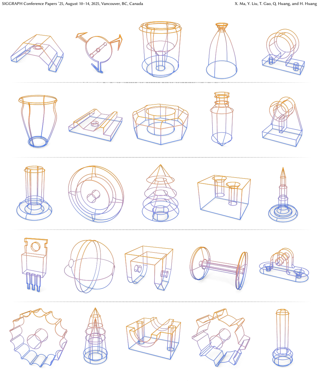
The central machinery is the wireframe VAE plus latent flow matching. In the curve stage, each curve is translated, rotated, and scaled so its endpoints sit at $[-1,0,0]$ and $[1,0,0]$, sampled to 256 points, reduced to 64 points by cross-attention, and compressed to a $4\times 3$ latent; decoding queries the latent with a positional embedding of $t$ through cross-attention, so one latent answers for every point along the curve. In the wireframe stage, the adjacency list is sorted by BFS and then rewritten as $\Delta Adj_V[i,0]=Adj_V[i,0]-Adj_V[i-1,0]$ and $\Delta Adj_V[i,1]=Adj_V[i,1]-Adj_V[i,0]$, reducing redundancy in the topology signal; a Perceiver encoder combines $Z_{\mathrm{Curve}}$, endpoint coordinates, and $\Delta Adj_V$ into $Z_W\in\mathbb{R}^{64\times 16}$. Flow matching trains a transformer velocity field $U_\theta(t,X_t,c)$ on this latent, with optional condition features from a point cloud or image encoder.

What would settle it

Take a wireframe graph that has several valid breadth-first orderings, or two disconnected components, and relabel its vertices; encode both versions with the trained wireframe VAE and decode them. If the two latents differ enough that the decoded wireframes are not isomorphic or clearly diverge, the representation is tracking an arbitrary vertex order rather than the graph itself, contradicting the claim that the latent encodes topology continuously.

Watch

Extended reading notes

Core claim

The authors claim that a wireframe's continuous curves and discrete connectivity can both live in a fixed-length continuous latent representation. Curves are normalized, sampled, and compressed into compact curve latents $Z_{\mathrm{Curve}}\in\mathbb{R}^{4\times 3}$; the decoder turns any query parameter $t$ into a 3D point on the curve, so the decoded object is a neural parametric curve rather than a fixed polyline. Topology is written as an adjacency list whose vertex indices are reordered by breadth-first search and then stored as differences, which makes the discrete structure more compressible. A perceiver-style attention VAE merges the curve latents, endpoint coordinates, and the differential adjacency list into a single $Z_W\in\mathbb{R}^{64\times 16}$, and a flow-matching model learns a velocity field that maps Gaussian noise to this latent. The paper concludes that joint encoding is the reason the model can generate irregular topologies, interpolate smoothly between wireframes with different topology, and reconstruct complete wireframes from sparse conditions.

Load-bearing premise

The load-bearing premise, stated in Sec. 3.2 and supplementary A.2, is that sorting a wireframe's vertices with a breadth-first search yields a consistent, canonical ordering, so the same wireframe always maps to the same latent regardless of the original vertex numbering; if that ordering is not reproducible, the differential adjacency code and the latent built from it are partly encoding an arbitrary traversal rather than the topology itself.

Editorial extensions

If this is right

On the filtered ABC test distribution, unconditional generation reports higher coverage, lower MMD, and better 1-NN accuracy than DeepCAD, BrepGen, and 3DWire under both Chamfer distance and EMD.
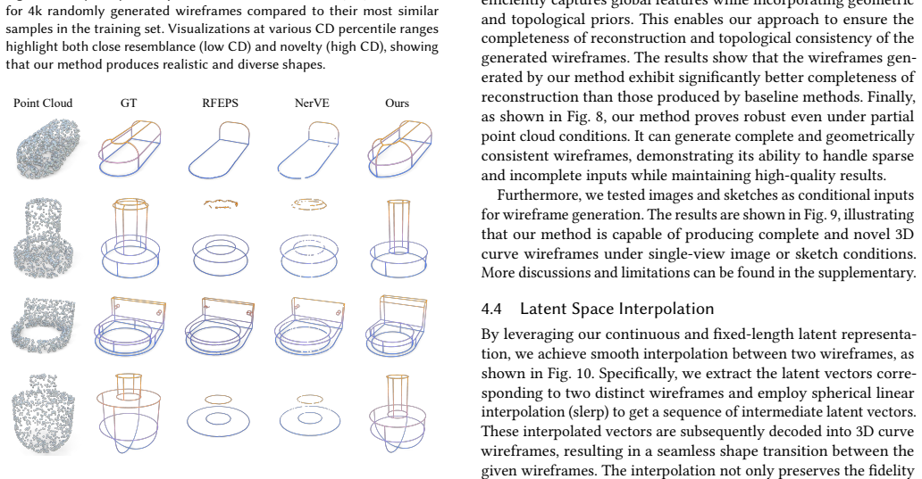
Conditional generation from point clouds works with 1,000 input points, versus 20,000 for the compared reconstruction methods, and reports lower Chamfer distance, lower EMD, and higher F-score on sparse inputs.
Because the latent is continuous and fixed-length, spherical interpolation between two wireframes with different topology yields intermediate shapes that change both geometry and connectivity, not just vertex positions.
The same trained flow-matching model accepts unconditional, point-cloud, image, and sketch conditioning, so the proposed representation is not tied to one input modality.
Ablation results tie the differential adjacency list and curve normalization to higher reconstruction accuracy and topology consistency, supporting the design as load-bearing rather than incidental.

Reading between the lines

Editorial extensions of the paper, not claims the author makes directly.

Inference: the fused-latent recipe should transfer to other mixed discrete/continuous 3D representations, such as B-rep edges and faces or skeleton graphs, where components are currently generated separately and stitched; a fused fixed-length latent would be a testable extension beyond the paper's wireframe setting.
Inference: the paper's own limitation note says conditional generation loses fine local detail, partly because the frozen image encoder was not trained on CAD data; fine-tuning that encoder on wireframe data is a concrete follow-up that could improve image- and sketch-conditioned results without changing the latent design.
Inference: the reported 7.3% of generated samples with new graph isomorphisms suggests the model can go beyond memorized topologies; a testable next step is conditioning explicitly on a target topology to control whether novelty is produced on demand.

Share X Bluesky LinkedIn Reddit HN

Signed reviews

No signed human review yet.

Editorial analysis

A structured set of objections, weighed in public.

Desk editor's note, referee report, and a circularity audit.

Desk Editor's Note

read the letter

Two things you should know. First, this is a real step forward for curve wireframe generation: a single fixed-length latent that encodes both curve geometry (as neural parametric curves) and topology (as a differential adjacency representation), with flow matching as the generative model. The ablations are convincing that each piece matters, and the unconditional generation numbers beat the cited baselines on COV, MMD, and 1-NN. Second, the main weak spot is the topology encoding. It relies on a BFS ordering of vertices that the paper never fully specifies: no root rule, no tie-breaking, no handling of disconnected components. BFS order is not unique for a typical wireframe graph, so the differential adjacency list is not invariant to vertex relabeling. That undermines part of the claim that the latent space is continuous with respect to topology, because the same wireframe can map to different latent codes depending on which valid BFS order happens to be produced. The paper's own limitation section reports 81.79% topology alignment, and it is unclear whether that metric is true graph isomorphism or just exact adjacency-list matching after the learned ordering. If it is the latter, reorderings are counted as failures, which would actually be good news; if it is the former, roughly 18% of samples have genuine topological errors. The paper does not tell us which. That is a fixable but important ambiguity. I also agree with the reader's other concerns: Table 1 has no error bars, the point-cloud comparison gives baselines 20K points while the proposed method gets 1K, and there is no code release. These do not sink the central idea, but they make the empirical claims weaker than the abstract suggests. On the plus side, the novelty is real relative to 3DWire, BrepGen, and DeepCAD, which decouple geometry and topology, and the interpolation results look like more than cherry-picking. The self-citation to 3DWire is fine; it is used as a baseline. Overall, the central argument holds up in the sense that the proposed representation is plausible and the experiments mostly support it, but the topology-ordering issue deserves a direct response from the authors before I would trust the continuity claim. For a reading group, the paper is worth discussing precisely because of the BFS question. I would cite it if I worked on wireframe or CAD generation, and I would take it seriously as a SIGGRAPH submission. Recommendation: send it to peer review, not desk reject. The right referees will push for a precise definition of the topology metric and, ideally, a canonical ordering or a permutation-invariant alternative.

Referee Report

5 major / 5 minor

Summary. The paper proposes CLR-Wire, a framework that encodes 3D curve wireframes into a continuous fixed-length latent space by combining a curve VAE with a wireframe VAE that ingests geometry (neural parametric curves and vertex coordinates) and topology (a differential adjacency list). A flow-matching model generates these latents either unconditionally or conditioned on point clouds, images, or sketches. The authors report improved COV/MMD/1-NN over DeepCAD, BrepGen, and 3DWire on a filtered ABC dataset, improved CD/EMD/F-score over RFEPS and NerVE on sparse point-cloud conditional reconstruction, and demonstrate latent interpolation and downstream applications.

Significance. If the reported results are reproducible, the paper makes a useful contribution to generative modeling of CAD wireframes: it is a plausible step toward joint modeling of geometry and topology in a continuous latent space, with a clean flow-matching formulation and extensive ablations supporting the design choices (normalization, differential adjacency, latent dimension). The framework is flexible, supporting multiple conditioning modalities. The reported unconditional-generation gains are large (for example, 1-NN 54.10% versus 64.49% for 3DWire), which would be meaningful if confirmed. The strengths include detailed training and implementation details, reproducible experimental settings, and a substantial supplementary evaluation with ablations and failure-mode analysis.

major comments (5)

[Sec. 3.2 / Supp. A.2] The topology encoding is not invariant to vertex relabeling because the BFS traversal is underspecified: no root selection rule, no neighbor tie-breaking rule, and no handling of disconnected components are given. Since the differential adjacency list ΔAdj_V is read from this ordering, the latent representation Z_W encodes an arbitrary ordering rather than the graph itself. Moreover, with only 6 column-difference and 24 row-difference categories while Fig. 13 shows out-of-range values, the encoding is also lossy, and the paper does not state how out-of-range values are treated. This undermines the claim that Z_W is a continuous latent representation of topology, and it means the reported 81.79% topology alignment on generated samples cannot distinguish reordering mismatches from genuine topological errors.
[Sec. 4 / Supp. B.2 / Sec. D] The central claim of joint geometry/topology generation is not directly quantified: Table 1 reports only point-based geometric metrics (COV/MMD/1-NN computed on sampled points), while the sole topology metric for generated samples, 81.79% in Section D, is defined inconsistently with the 'isomorphic' definition in Supplementary B.2 that is used for Table 4's Topo. column. The reader cannot tell whether the 81.79% reflects true topological failures or non-canonical orderings, and the gap between this generation-time value and the 99.91% reconstruction-time Topo. in Table 4 is unexplained. The main paper should report a clearly defined topology metric on generated samples, together with error bars, to support the claimed improvements in topology modeling.
[Sec. 4.2 / Table 1] The unconditional comparison is not fully controlled: DeepCAD and BrepGen are evaluated using their pretrained models, which were trained on different data distributions, while 3DWire is retrained on the authors' filtered ABC dataset. This asymmetry can bias the quantitative results, because the baselines are not given the same training distribution. The authors should either retrain all baselines on the same filtered dataset or justify why the transfer protocol is appropriate for a fair comparison.
[Sec. 4.3 / Table 2] The point-cloud conditional comparison is unfair: RFEPS and NerVE receive dense 20K-point inputs, whereas CLR-Wire receives only 1K sparse points, and no details are given on whether the baselines were retrained on the authors' data or evaluated on the same test set. The reported superiority may reflect input difficulty rather than method quality. The comparison should be repeated with matched input conditions (for example, the same 1K-point inputs for all methods) or the authors should clearly frame the result as an advantage in data efficiency rather than a head-to-head accuracy comparison.
[Sec. 4.2 / Tables 1 and 2] No variance or confidence intervals are reported for COV, MMD, 1-NN, CD, EMD, or F-score, despite the statement that 10 independent random samplings of 2k generated samples were performed. Without error bars (or at least standard deviations across the 10 samplings), the claimed 'substantial improvements' cannot be assessed for statistical significance, and some gaps in Table 2 are small relative to plausible sampling noise.

minor comments (5)

[Supp. A.1] There are typos in the supplementary: 'normailze' and 'paramatric' should be 'normalize' and 'parametric'.
[Fig. 10 caption] The caption contains garbled characters ('čaĎ', 'čbĎ', 'čcĎ', etc.) that should be corrected to the proper roman-numeral labels.
[Supp. A.2 / Table 4] The terms 'Difference Adjacency' and 'Differential Adjacency' are used interchangeably; one consistent term should be adopted.
[Table 4] The row labels A/B/C for the ablation settings are not explained in the caption; the caption should explicitly state which rows correspond to which configuration (for example, which setting is the default).
[Supp. B.2] The Corner Chamfer Distance (CCD) metric is used in Table 4 but is not formally defined in the metrics section; a definition should be added.

Circularity Check

0 steps flagged · score 0.0 of 10

No circularity found: the central latent-representation and flow-matching results are evaluated against external baselines and a held-out test split; the only same-group citation is a baseline and a preprocessing convention, not load-bearing.

full rationale

The paper's derivation chain is self-contained in the relevant sense. The curve VAE compresses normalized curves into Z_Curve and reconstructs them via a parametric query t; the wireframe VAE combines Z_Curve, V_Coords, and Adj_V into a fixed-length latent Z_W and is trained against reconstruction losses; the flow-matching model maps Gaussian noise to Z_W and is evaluated by generating samples and comparing them with a held-out test set using COV, MMD, and 1-NN against external baselines DeepCAD, BrepGen, 3DWire, RFEPS, and NerVE. No claimed prediction is produced by fitting a parameter to a subset and then reporting a closely related quantity as a prediction; the quantitative claims rest on held-out comparisons. The differential adjacency list is an encoding transformation of the adjacency list, not a result derived from itself, and its discretization into 6 column-difference and 24 row-difference categories is an implementation detail whose limitations are acknowledged. The BFS-assisted vertex ordering is a potential correctness and robustness concern, since BFS ordering is not canonical, but that is an external, testable assumption about the representation, not a circular reduction: the paper does not define topology consistency in terms of the BFS ordering and does not use the ordering's existence as evidence for its generation claims. The same-group citation to 3DWire appears as a baseline in Table 1 and as the source of the z-y-x then BFS vertex sorting convention in Supplementary A.2; neither use is load-bearing for the central latent-space contribution, and the 3DWire baseline is retrained on the paper's curve-wireframe dataset rather than used to justify the method's validity. The disclosed limitation that only 81.79% of generated samples achieve topological alignment, measured by adjacency list and vertex consistency, weakens the strength of the topology-consistency claim but is an honest reported metric, not a circular step. Accordingly, no specific reduction from an output to an input by construction or by self-citation can be exhibited, and the appropriate circularity score is 0.

Assumptions & free parameters 5 free parameters · 5 assumptions · 0 invented entities

The paper introduces no new physical entities, forces, or conserved quantities. 'Neural Parametric Curves' and the differential adjacency list are learned representations and encodings, not independent postulated entities. The main assumptions are domain-level: distinct curve endpoints, canonical BFS ordering, and the sufficiency of a fixed-size latent on a filtered dataset.

free parameters (5)

Wireframe latent dimension (Z_W) = 64x16 (16 channels)
Size of the fixed-length continuous latent; Table 4 shows reconstruction error drops as dimension rises from 4 to 16, so the choice is a capacity knob for the central claim.
Curve VAE KL weight = 5e-6
Hand-set regularization weight; balances reconstruction versus latent smoothness for flow matching.
Wireframe VAE KL weight = 5e-5
Hand-set regularization weight controlling the prior alignment of Z_W.
Differential adjacency categories = Col Diff 6, Row Diff 24
Discretization of the differential adjacency values; imposes a fixed vocabulary for topology prediction, a hand-set assumption that limits representable graphs.
Maximum curves per wireframe (M) = 128 (implied by data filter)
Decoder uses M learnable queries; samples with more than 128 curves were removed, so the method targets only wireframes within this range.

assumptions (5)

standard math VAE reparameterization and KL regularization produce a smooth continuous latent space that flow matching can model.
Sec. 3.2 and A.3 rely on standard VAE and flow matching theory to justify the latent and the generative trajectory.
domain assumption Curve normalization requires distinct start and end points; closed curves are not explicitly handled.
Sec. 3.1 and supplementary A.1 define rotation using the endpoint vector p'_n; a closed curve with p'_n = 0 makes the rotation axis undefined.
domain assumption BFS traversal yields a canonical, consistent ordering of vertices for the differential adjacency list.
Sec. 3.2 and A.2 use BFS sorting to define the adjacency encoding; BFS is non-unique and incomplete for disconnected graphs, so the ordering is not a topological invariant.
domain assumption Wireframes with at most 128 curves and from single solids, after filtering, define the target distribution.
Sec. 4.1 filters out multi-solid samples, simple shapes, and samples with more than 128 curves, so the claimed generality applies only to this filtered subset.
domain assumption Fixed-length latent Z_W (64x16) is sufficient to reconstruct up to M curves without losing critical topology or geometry.
Sec. 3.2 decodes all M possible curves from the same fixed latent; Table 4 shows higher latent dimension improves reconstruction, so the chosen dimension is a real bottleneck.

how reviews work

0 comments

Cite this review

Pith. "Pith review of CLR-Wire: Towards Continuous Latent Representations for 3D Curve Wireframe Generation." pith.science (2026). https://pith.science/paper/6D7SBRLU

@misc{pith2026250419174,
  author       = {Pith},
  title        = {Pith review of: CLR-Wire: Towards Continuous Latent Representations for 3D Curve Wireframe Generation},
  year         = {2026},
  howpublished = {\url{https://pith.science/paper/6D7SBRLU}},
  note         = {Machine review of arXiv:2504.19174}
}

read the original abstract

We introduce CLR-Wire, a novel framework for 3D curve-based wireframe generation that integrates geometry and topology into a unified Continuous Latent Representation. Unlike conventional methods that decouple vertices, edges, and faces, CLR-Wire encodes curves as Neural Parametric Curves along with their topological connectivity into a continuous and fixed-length latent space using an attention-driven variational autoencoder (VAE). This unified approach facilitates joint learning and generation of both geometry and topology. To generate wireframes, we employ a flow matching model to progressively map Gaussian noise to these latents, which are subsequently decoded into complete 3D wireframes. Our method provides fine-grained modeling of complex shapes and irregular topologies, and supports both unconditional generation and generation conditioned on point cloud or image inputs. Experimental results demonstrate that, compared with state-of-the-art generative approaches, our method achieves substantial improvements in accuracy, novelty, and diversity, offering an efficient and comprehensive solution for CAD design, geometric reconstruction, and 3D content creation.

Figures

Figures reproduced from arXiv: 2504.19174 by the authors.

**Figure 1.** Our approach encodes discrete topological structures and continuous geometric information into a unified Continuous Latent Representation, enabling [PITH_FULL_IMAGE:figures/full_fig_p001_1.png] view at source ↗

**Figure 2.** Overview of wireframe generation. Our method employs Latent Flow Matching based on the proposed latent wireframe representation 𝑍𝑊 , which is decoded into a wireframe via the Wireframe Decoder. First, random noise is mapped to 𝑍𝑊 , and then decoded into adjacency Adj𝑉 , endpoint coordinates 𝑉Coords, and curve latents 𝑍Curve. The final wireframe is produced using Adj𝑉 , 𝑉Coords, and 3D curves decoded from 𝑍Curve. Fur… view at source ↗

**Figure 3.** 2D Curve normalization examples. Curves are normalized successively through translation, rotation, and scaling to align their start and end points, ensuring consistent spatial representation. Loss functions. During training, we optimize the Wireframe VAE using three loss functions: 1) MSE loss for curve latent representations 𝑍Curve and vertex coordinates 𝑉Coords; 2) cross-entropy loss for predicting the adjacency… view at source ↗

Figures from the paper (24 more)

**Figure 4.** Figure 4: Wireframe VAE pipeline. Given a 3D curve wireframe, we extract curve latents 𝑍Curve from normalized curves via Curve Encoder, and the topology embeddings, which include adjacency Adj𝑉 embeddings and corresponding vertex coordinate 𝑉Coords embeddings. They are concatena…

**Figure 5.** Figure 5: Qualitative evaluation of our method with state-of-the-art methods, BrepGen[Xu et al [PITH_FULL_IMAGE:figures/full_fig_p006_5.png]

**Figure 8.** Figure 8: Visualization examples under the partial point cloud condition. By [PITH_FULL_IMAGE:figures/full_fig_p007_8.png]

**Figure 7.** Figure 7: Comparison with RFEPS [Xu et al. 2022] and NerVE [Zhu et al. 2023] under the sparse point cloud condition. Our method achieves competitive results even with fewer points. detecting sharp edges to reconstruct wireframe structures. However, for objects with smoother sur…

**Figure 9.** Figure 9: Visualization examples under single-view image and sketch conditions. [PITH_FULL_IMAGE:figures/full_fig_p010_9.png]

**Figure 10.** Figure 10: Visualization examples for latent interpolation. (b)-(e) show continuous transitions between shapes with different topologies. Specifically, (e) illustrates [PITH_FULL_IMAGE:figures/full_fig_p010_10.png]

**Figure 11.** Figure 11: Visualization examples of unconditional wireframe generation. Our method is capable of generating high-quality wireframes with complex topological [PITH_FULL_IMAGE:figures/full_fig_p011_11.png]

**Figure 12.** Figure 12: CurveVAE training pipeline: Input curves are sampled and posi [PITH_FULL_IMAGE:figures/full_fig_p012_12.png]

**Figure 13.** Figure 13: Distribution of wireframe vertex counts, row differences (Row Diff ) [PITH_FULL_IMAGE:figures/full_fig_p012_13.png]

**Figure 14.** Figure 14: The construction process of the differential adjacency list [PITH_FULL_IMAGE:figures/full_fig_p013_14.png]

**Figure 15.** Figure 15: The wireframe is mapped to the latent space using Curve and [PITH_FULL_IMAGE:figures/full_fig_p013_15.png]

**Figure 16.** Figure 16: Ablation study on the wireframe reconstructed by (a) removing [PITH_FULL_IMAGE:figures/full_fig_p015_16.png]

**Figure 17.** Figure 17: Visualization of the impact of different latent space dimensions [PITH_FULL_IMAGE:figures/full_fig_p015_17.png]

**Figure 19.** Figure 19: The resulting wireframe can be converted into a mesh model. [PITH_FULL_IMAGE:figures/full_fig_p015_19.png]

**Figure 20.** Figure 20: Four common failure cases categories for our method. [PITH_FULL_IMAGE:figures/full_fig_p016_20.png]

**Figure 21.** Figure 21: Unconditional wireframe generation of different methods. [PITH_FULL_IMAGE:figures/full_fig_p017_21.png]

**Figure 22.** Figure 22: Unconditional wireframe generation of different methods. [PITH_FULL_IMAGE:figures/full_fig_p018_22.png]

**Figure 23.** Figure 23: Wireframe novelty analysis. For each random wireframe generated by our method, we show the top four most similar wireframes retrieved from the [PITH_FULL_IMAGE:figures/full_fig_p019_23.png]

**Figure 24.** Figure 24: Latent Space Interpolation. 20 [PITH_FULL_IMAGE:figures/full_fig_p020_24.png]

**Figure 25.** Figure 25: More results for sparse point cloud condition generation. [PITH_FULL_IMAGE:figures/full_fig_p021_25.png]

**Figure 26.** Figure 26: More results for partial point cloud condition generation. [PITH_FULL_IMAGE:figures/full_fig_p022_26.png]

**Figure 27.** Figure 27: More results for single-view image and sketch condition generation. [PITH_FULL_IMAGE:figures/full_fig_p023_27.png]

**Figure 28.** Figure 28: More results for unconditional wireframe generation. [PITH_FULL_IMAGE:figures/full_fig_p024_28.png]

**Figure 29.** Figure 29: More results for unconditional wireframe generation (cont.). [PITH_FULL_IMAGE:figures/full_fig_p025_29.png]

Discussion (0). Continue with ORCID to comment.

Forward citations

Cited by 1 Pith paper

Reviewed papers in the Pith corpus that reference this work. Sorted by Pith novelty score. Full citation record

Auto-Regressive Surface Cutting
cs.GR 2025-06 conditional novelty 6.0 of 10

SeamGPT generates artist-style mesh cutting seams as auto-regressively predicted quantized 3D line segments, improving UV unwrapping and part segmentation.

Reference graph

Works this paper leans on

12 extracted references · 10 canonical work pages · cited by 1 Pith paper

[1]

The new set of curve points is represented as: P′ = P−𝑝1

Translation: Shift the starting point𝑝1 of the polyline to(0, 0, 0) to eliminate the influence of the initial position. The new set of curve points is represented as: P′ = P−𝑝1

work page
[2]

Using Rodrigues’ rotation, we construct the rotation matrix R: R = I+ sin𝜃 K+( 1− cos𝜃)K2, where K is the skew-symmetric matrix derived from the rotation axis vector a

Rotation: Align the end vector of the curve p′𝑛 =𝑝𝑛−𝑝1 with the target direction vector(1, 0, 0). Using Rodrigues’ rotation, we construct the rotation matrix R: R = I+ sin𝜃 K+( 1− cos𝜃)K2, where K is the skew-symmetric matrix derived from the rotation axis vector a. The rotation axis a is calculated as: a = p′𝑛×( 1, 0, 0) ∥p′𝑛×( 1, 0, 0)∥, and the skew-sy...

work page
[3]

The scaling factor is calculated as: 𝑠 = 2 p′′𝑛[0]

Scaling: Scale the set of points so that the x-coordinate of the endpoint becomes 1. The scaling factor is calculated as: 𝑠 = 2 p′′𝑛[0]. After scaling, the set of points on the curve is: P′′ =𝑠·( R· P′)−( 1, 0, 0). Through these steps, the curve is normalized to a standard form with the starting point at(−1, 0, 0) and the endpoint at(1, 0, 0). Training. W...

work page 2016
[7]

DeepLSD: Line Segment Detection and Refinement with Deep Image Gradients. In Proc. IEEE/CVF Conf. on Computer Vision & Pattern Recognition . 17327–17336. 8 CLR-Wire: Towards Continuous Latent Representations for 3D Curve Wireframe Generation SIGGRAPH Conference Papers ’25, August 10–14, 2025, Vancouver, BC, Canada William Peebles and Saining Xie. 2023. Sc...

work page 1982
[8]

NEAT: Distilling 3D Wireframes from Neural Attraction Fields. In Proc. IEEE/CVF Conf. on Computer Vision & Pattern Recognition . 19968–19977. Nan Xue, Tianfu Wu, Song Bai, Fu-Dong Wang, Gui-Song Xia, Liangpei Zhang, and Philip H. S. Torr. 2023. Holistically-Attracted Wireframe Parsing: From Supervised to Self-Supervised Learning. IEEE Trans. Pattern Anal....

work page 2023
[9]

NerVE: Neural Volumetric Edges for Parametric Curve Extraction from Point Cloud. In Proc. IEEE/CVF Conf. on Computer Vision & Pattern Recognition . 13601– 13610. Yixin Zhuang, Ming Zou, Nathan Carr, and Tao Ju. 2013. A general and efficient method for finding cycles in 3D curve networks. ACM Trans. Graph. 32, 6, Article 180 (Nov. 2013), 10 pages. 9 SIGGRA...

work page 2013
[2015]

ACM Trans

Flow aligned surfacing of curve networks. ACM Trans. Graph. 34, 4, Article 127 (July 2015), 10 pages. Jeong Joon Park, Peter R. Florence, Julian Straub, Richard A. Newcombe, and Steven Lovegrove. 2019. DeepSDF: Learning Continuous Signed Distance Functions for Shape Representation. In Proc. IEEE/CVF Conf. on Computer Vision & Pattern Recog- nition. 165–17...

work page 2015
[2017]

ACM Trans

FlowRep: descriptive curve networks for free-form design shapes. ACM Trans. Graph. 36, 4, Article 59 (2017), 14 pages. Haoxiang Guo, Shilin Liu, Hao Pan, Yang Liu, Xin Tong, and Baining Guo. 2022. Com- plexGen: CAD reconstruction by B-rep chain complex generation. ACM Trans. on Graphics (Proc. SIGGRAPH) 41, 4 (2022), 129:1–129:18. Kaiming He, Xiangyu Zhan...

work page 2017

Show all 12 references

[2018]

Learning to Parse Wireframes in Images of Man-Made Environments. In Proc. IEEE/CVF Conf. on Computer Vision & Pattern Recognition . 626–635. Shangfeng Huang, Ruisheng Wang, Bo Guo, and Hongxin Yang. 2024. PBWR: Parametric-Building-Wireframe Reconstruction from Aerial LiDAR Poi...

2023
[2022]

Learning to Construct 3D Building Wireframes from 3D Line Clouds. In Proc. British Machine Vision Conference . 91. Wenchao Ma, Bin Tan, Nan Xue, Tianfu Wu, Xianwei Zheng, and Gui-Song Xia. 2022. HoW-3D: Holistic 3D Wireframe Perception from a Single Image. InInt. Conf. on 3D V...

2022
[2023]

arXiv:2312.11417 [cs.CV] Li Cao, Yike Xu, Jianwei Guo, and Xiaoping Liu

PolyDiff: Generating 3D Polygonal Meshes with Diffusion Models. arXiv:2312.11417 [cs.CV] Li Cao, Yike Xu, Jianwei Guo, and Xiaoping Liu. 2023. WireframeNet: A novel method for wireframe generation from point cloud. Comput. Graph. 115 (2023), 226–235. Jiacheng Chen, Ruizhi Deng...

2023 arXiv
[2024]

arXiv:2406.10853 [cs.CV] Jingyu Hu, Ka-Hei Hui, Zhengzhe Liu, Ruihui Li, and Chi-Wing Fu

MV2Cyl: Reconstructing 3D Extrusion Cylinders from Multi-View Images. arXiv:2406.10853 [cs.CV] Jingyu Hu, Ka-Hei Hui, Zhengzhe Liu, Ruihui Li, and Chi-Wing Fu. 2024. Neural Wavelet-domain Diffusion for 3D Shape Generation, Inversion, and Manipulation. ACM Trans. Graph. 43, 2 (...

2024 arXiv

Pith tools

Reviewed August 16, 2026 · model on record in the stance chip above.

[1] [1]

The new set of curve points is represented as: P′ = P−𝑝1

Translation: Shift the starting point𝑝1 of the polyline to(0, 0, 0) to eliminate the influence of the initial position. The new set of curve points is represented as: P′ = P−𝑝1

work page

[2] [2]

Using Rodrigues’ rotation, we construct the rotation matrix R: R = I+ sin𝜃 K+( 1− cos𝜃)K2, where K is the skew-symmetric matrix derived from the rotation axis vector a

Rotation: Align the end vector of the curve p′𝑛 =𝑝𝑛−𝑝1 with the target direction vector(1, 0, 0). Using Rodrigues’ rotation, we construct the rotation matrix R: R = I+ sin𝜃 K+( 1− cos𝜃)K2, where K is the skew-symmetric matrix derived from the rotation axis vector a. The rotation axis a is calculated as: a = p′𝑛×( 1, 0, 0) ∥p′𝑛×( 1, 0, 0)∥, and the skew-sy...

work page

[3] [3]

The scaling factor is calculated as: 𝑠 = 2 p′′𝑛[0]

Scaling: Scale the set of points so that the x-coordinate of the endpoint becomes 1. The scaling factor is calculated as: 𝑠 = 2 p′′𝑛[0]. After scaling, the set of points on the curve is: P′′ =𝑠·( R· P′)−( 1, 0, 0). Through these steps, the curve is normalized to a standard form with the starting point at(−1, 0, 0) and the endpoint at(1, 0, 0). Training. W...

work page 2016

[4] [7]

DeepLSD: Line Segment Detection and Refinement with Deep Image Gradients. In Proc. IEEE/CVF Conf. on Computer Vision & Pattern Recognition . 17327–17336. 8 CLR-Wire: Towards Continuous Latent Representations for 3D Curve Wireframe Generation SIGGRAPH Conference Papers ’25, August 10–14, 2025, Vancouver, BC, Canada William Peebles and Saining Xie. 2023. Sc...

work page 1982

[5] [8]

NEAT: Distilling 3D Wireframes from Neural Attraction Fields. In Proc. IEEE/CVF Conf. on Computer Vision & Pattern Recognition . 19968–19977. Nan Xue, Tianfu Wu, Song Bai, Fu-Dong Wang, Gui-Song Xia, Liangpei Zhang, and Philip H. S. Torr. 2023. Holistically-Attracted Wireframe Parsing: From Supervised to Self-Supervised Learning. IEEE Trans. Pattern Anal....

work page 2023

[6] [9]

NerVE: Neural Volumetric Edges for Parametric Curve Extraction from Point Cloud. In Proc. IEEE/CVF Conf. on Computer Vision & Pattern Recognition . 13601– 13610. Yixin Zhuang, Ming Zou, Nathan Carr, and Tao Ju. 2013. A general and efficient method for finding cycles in 3D curve networks. ACM Trans. Graph. 32, 6, Article 180 (Nov. 2013), 10 pages. 9 SIGGRA...

work page 2013

[7] [2015]

ACM Trans

Flow aligned surfacing of curve networks. ACM Trans. Graph. 34, 4, Article 127 (July 2015), 10 pages. Jeong Joon Park, Peter R. Florence, Julian Straub, Richard A. Newcombe, and Steven Lovegrove. 2019. DeepSDF: Learning Continuous Signed Distance Functions for Shape Representation. In Proc. IEEE/CVF Conf. on Computer Vision & Pattern Recog- nition. 165–17...

work page 2015

[8] [2017]

ACM Trans

FlowRep: descriptive curve networks for free-form design shapes. ACM Trans. Graph. 36, 4, Article 59 (2017), 14 pages. Haoxiang Guo, Shilin Liu, Hao Pan, Yang Liu, Xin Tong, and Baining Guo. 2022. Com- plexGen: CAD reconstruction by B-rep chain complex generation. ACM Trans. on Graphics (Proc. SIGGRAPH) 41, 4 (2022), 129:1–129:18. Kaiming He, Xiangyu Zhan...

work page 2017